
I first met Brownian motion in a fluid dynamics course at UCL, long before I had any reason to care about option prices, and it is still slightly strange to me that the same mathematics describes pollen grains in water and the price of Bitcoin. It does, though, and understanding why is the quickest route I know into how quantitative finance actually thinks about prices. This post is the physics first, then the finance, then the equations that connect them.
The physics
In 1827 the botanist Robert Brown looked at pollen grains suspended in water under a microscope and saw them jittering about with no apparent cause. It took until 1905 for Einstein to explain it: the grains were being knocked around by water molecules, far too small to see, hitting them from random directions many times a second. Each individual collision is tiny. The sum of millions of them is a visible random walk.
Three things follow from that picture, and all three carry over to markets. First, the path is a random walk: the direction of the next step has nothing to do with the direction of the last one. Second, how far a particle wanders depends on a single number, the diffusion coefficient, which in turn depends on the temperature of the fluid, its viscosity, and the size of the particle. Hotter, thinner fluid and smaller particles mean more wandering. Third, the distance travelled does not grow in proportion to time. The mean squared displacement grows linearly with time, which means the typical distance grows with the square root of time. Wait four times as long and a particle has wandered twice as far, not four times.
Engineers use this every day. Diffusion in chemical reactors, the behaviour of aerosols in air filtration, how a drug spreads through tissue, the mixing of one fluid into another: all of it rests on the same equations, and the diffusion coefficient is the number you measure or calculate first.
The finance
The first person to apply this to prices was not a physicist but a French mathematician, Louis Bachelier, who modelled stock prices on the Paris exchange as a random walk in 1900, five years before Einstein’s paper. The idea sat largely ignored for half a century and then became the foundation of modern quantitative finance.
The correspondence is close. A price moves because of a very large number of small, more or less independent decisions by buyers and sellers, which plays the role of the molecular collisions. Volatility plays the role of the diffusion coefficient: it is the single number that says how far the price tends to wander in a given time. And the square-root-of-time rule carries over exactly, which is why volatility is quoted annualised and then scaled by the square root of the horizon when you want the expected move over a month or a week. I used that rule in the Bitcoin option post without explaining where it came from. This is where it comes from.
Once you accept the analogy, a whole toolkit arrives with it. Stochastic differential equations, which engineers use to describe a particle under random forcing, describe a price path with a drift term for the average return and a diffusion term for the volatility, and Black-Scholes is derived from exactly such an equation. Monte Carlo simulation, which is how you study diffusion when the geometry is too awkward for an analytical solution, is also how you price a complicated derivative or stress a portfolio: generate thousands of random price paths and look at the distribution of outcomes. And mean reversion, where a restoring force pulls a particle back toward an equilibrium position, has a direct financial counterpart in the Ornstein-Uhlenbeck process, which is used for interest rates and for commodity spreads that tend to return to a long-run level.
The equations
Standard Brownian motion in one dimension is a process B(t) whose value at time t is normally distributed with mean zero and variance t:
\[B(t) \sim N(0, t)\]The variance growing with t is the square-root-of-time rule in its mathematical form. The increments over any interval are independent of what came before and are themselves normal, with variance equal to the length of the interval:
\[B(t + s) – B(t) \sim N(0, s)\]That is the random walk with no bias in either direction. To describe something that drifts as well as wanders, you add a deterministic term. Written as a stochastic differential equation, the change in X over a small time step is
\[dX_t = \mu\, dt + \sigma\, dB_t\]where μ is the drift, the average movement per unit time, and σ is the volatility, the size of the random part. In the physics μ would be a steady current carrying the particle along and σ would be the diffusion coefficient.
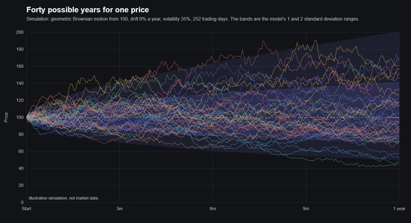
For prices there is one more step. A price cannot go below zero, and a move of £5 means something different on a £10 stock than on a £500 one, so the natural thing to model is the proportional change rather than the absolute one. That gives geometric Brownian motion, in which the price at time t is
\[S_t = S_0\, e^{\left(\mu – \frac{1}{2}\sigma^2\right)t + \sigma B_t}\]where S0 is the starting price. Because the random part sits in the exponent, the price stays positive, and the log of the price follows ordinary Brownian motion with drift. That is the model Black-Scholes assumes, and it is why the volatility calculations in my earlier posts use log returns: under this model it is the log returns, not the prices, that are normally distributed. The slightly odd half-sigma-squared term in the drift is a correction that comes out of the calculus of random processes, and it is there so that μ really is the average growth rate of the price rather than of its logarithm.
Where the analogy stops
It is worth saying plainly that prices are not pollen grains. Molecular collisions really are independent and really are normally distributed in aggregate, because there are so many of them. Trades are not. People react to each other, volatility clusters so that wild days follow wild days, and the extreme moves happen far more often than the normal distribution allows, which I showed with a year of real Bitcoin data in an earlier post. Geometric Brownian motion is the starting point for every pricing model precisely because it is simple, and every serious model since has been an attempt to patch the ways in which it is wrong. But you have to understand the starting point before the patches make sense, and the quickest way to understand it is to remember that it was a description of physics first.