
Most people who trade for a living end up on one side of a divide they did not know existed when they started. On one side are directional traders, who have a view about where something is going and put money behind it. On the other are relative value traders, who try not to have a view about direction at all and make their money from the gap between two prices that ought to be related. I have done both, and the experience of moving between them taught me more about risk than anything else in my career.
The difference is easier to see in numbers than in description, so after setting the two out I run both over sixteen years of Brent and WTI crude prices.
Directional trading
Directional trading is what people imagine trading to be. You think oil is going down, you sell oil futures. You think a company will beat its numbers, you buy the shares. You think the index will rally, you buy calls. The analysis behind the view might be macroeconomic, or fundamental, or technical, or some mix, but the shape of the position is always the same: you are long or short something, and you win if the market goes your way.
The appeal is obvious. When you are right the payoff is clean, and there is no cap on how right you can be. The problem is that you are exposed to the whole market every minute you hold the position. If the index drops 3 per cent on something that has nothing to do with your view, your position drops with it, and your careful analysis of the company’s prospects does not help.
So the risk management for directional trading is about limiting how much the market can take from you before you concede. A stop at a sensible distance, sized to the volatility of the asset, so that ordinary noise does not trigger it and a real move does. Position sizes that mean no single trade can do serious harm to the account. Some diversification across assets that do not move together, with the caveat from my correlation post that in a crash they all do. A habit of checking that the potential gain is a multiple of the potential loss before putting the trade on, not after. And, where it makes sense, an option or a futures hedge that caps the downside on the part of the risk you did not want.
Relative value trading
Relative value is the other way of thinking. Instead of asking whether something will go up, you ask whether two things are priced correctly against each other, and if not, you buy the cheap one and sell the expensive one. The classic example is a pair of similar companies: if Ford looks cheap against General Motors by whatever measure you trust, you go long Ford and short GM, and you make money if the gap closes, whether the car industry as a whole goes up, down or sideways. The same logic runs through the yield curve, where you might buy ten-year bonds and sell two-year bonds if you expect the curve to flatten, and through statistical arbitrage, where a model finds dozens of such gaps and trades them all at once.
The attraction is that you have largely removed the market from the equation. A pairs trade has little beta; a crash hurts both legs and the losses mostly cancel. That is why relative value desks can run with much more leverage than directional ones, and why their returns, in normal times, look so smooth.
The catch is in the phrase “in normal times”. A relative value trade is a bet that a relationship holds, and relationships in markets are not laws of physics. The spread you are trading can widen before it narrows, and it can keep widening for longer than your capital lasts. Two assets that have moved together for ten years can stop doing so because of a takeover, a regulatory change or simply because everyone else was in the same trade and had to get out at once. And because the positions are leveraged, a spread that moves against you by a small amount in price terms can be a large amount in money terms.
So the risk management is different in kind. You need a stop on the spread itself, not on either leg, with a clear number at which you accept that the relationship has broken rather than merely stretched. You need to watch the correlation between the two legs continuously rather than assuming it from history. You need to be honest about liquidity, because a spread that takes months to close ties up capital for months, and the leverage that looked prudent at the start looks less so if you are still waiting in the fourth month. And you need many trades rather than one, so that a single relationship breaking does not take the book with it.
Side by side
| Directional | Relative value | |
|---|---|---|
| What you are betting on | The price of one thing goes up or down | The gap between two prices closes |
| Exposure to the market | High | Low in normal times |
| Where the profit comes from | The asset moving your way | The spread converging |
| Typical leverage | Moderate | Higher, because the market risk is hedged |
| What kills you | Being wrong and not getting out | The relationship breaking, or running out of time |
| Main risk tools | Stops, sizing, hedges | Spread stops, correlation monitoring, many small trades |
Brent against WTI: one relationship, sixteen years
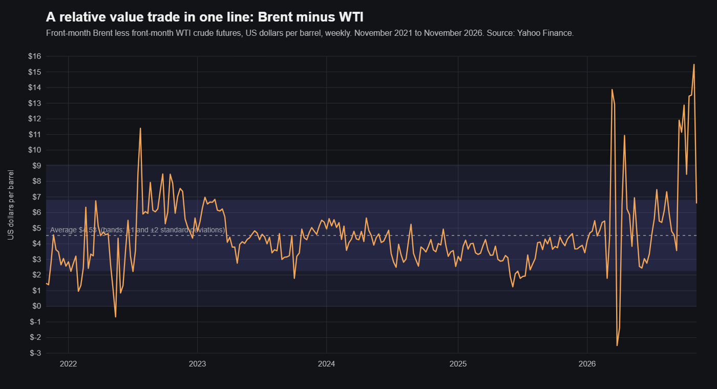
Brent and WTI are two grades of light crude oil, one priced off the North Sea and one delivered at Cushing, Oklahoma. They are close enough substitutes that their prices move together, and different enough in where and how they are delivered that the gap between them moves as well. That makes the pair a clean way to compare the two styles: a directional trader holds one of them, a relative value trader holds the difference.
I took weekly closes of the front-month futures for both, from January 2010 to the end of October 2026, 879 weeks in all, from Yahoo Finance.
| Brent | Brent minus WTI | |
|---|---|---|
| Volatility of weekly changes, annualised | $25.57 a barrel | $11.21 a barrel |
| Worst four weeks, held long | −$30.84 (to 13 March 2020) | −$15.06 (to 11 November 2011) |
| Average move for every $1 move in Brent | $1 | 12 cents |
The weekly changes in the two crudes had a correlation of 0.90, and the spread moved on average 12 cents for every dollar Brent moved, so almost all of the market’s direction does cancel out. What is left is still not small. The spread’s volatility was less than half of Brent’s, not a tenth of it, and its worst four weeks cost half as much per barrel as Brent’s worst four weeks, which came in the collapse of March 2020. Hedging out the direction removes the market from the trade. It does not remove the risk. It swaps one kind for another.
One technical point if you reproduce this. The two front-month contracts expire on different days, so for part of each month the spread compares oil for different delivery months, which adds noise around the roll dates. A desk trading the spread would hold the same delivery month on both legs.
When the relationship broke
At the end of 2010 the spread stood at $6.14 a barrel. Its average over the previous 52 weeks was $0.84 and its standard deviation $1.92, so it was 2.8 standard deviations above normal. On any statistical reading it was stretched, and the textbook trade was to sell it: short Brent, long WTI, and wait for the gap to close.
It did not close. Production from Canada and from the Bakken shale was arriving in the US Midwest faster than the pipelines out of Cushing could take it away, and WTI, which is priced at Cushing, fell behind the rest of the world. By the week of 7 October 2011 the weekly spread was $26.88, and the EIA recorded a daily high of $29.70 on 22 September. The spread averaged $0.94 in 2010, $15.96 in 2011 and $17.88 in 2012. It narrowed as new pipeline capacity reached the Gulf Coast from 2012, and again after the United States lifted its ban on crude exports at the end of 2015. Since 2016 it has averaged $4.39.
A trader who sold the spread at the end of 2010 and held on was $20.74 a barrel down at the worst point, about thirteen times the spread’s typical weekly move of $1.55. The position did eventually close at a small loss, after 45 weeks, but only because the average had risen to meet the spread: by November 2011 the 52-week average was $14.98. With the leverage spread trades usually carry, few books could have held it that long. This is what the relationship breaking means in practice. Nothing in the price history at the end of 2010 warned of it, because the cause was physical and it was new.
What the two styles look like in the data
To see the shape of each approach I ran two deliberately simple rules over the same 879 weeks, one barrel per trade, with no costs and no leverage.
The relative value rule trades the spread. When it is more than two standard deviations away from its 52-week average, it bets on a return to the average, and it closes at the average, at a spread stop four standard deviations against, or after 26 weeks, whichever comes first. The directional rule trades Brent alone: long when the price is above its 26-week average, short when it is below.
| Per barrel | Relative value (the spread) | Directional (Brent) |
|---|---|---|
| Trades | 30 | 99 |
| Share that made money | 70% | 22% |
| Average winner | $4.97 | $10.65 |
| Average loser | −$3.82 | −$3.85 |
| Best trade | $16.04 | $43.82 |
| Worst trade | −$8.38 | −$20.84 |
| Total over the period | $69.92 | −$62.30 |
The totals are the least interesting line. Change the settings and they change a lot: with a 13-week average the directional rule finishes $26 ahead, and with a 52-week average $39 behind. What does not change is the shape. Across those settings the directional rule wins on only 15 to 29 per cent of its trades and makes its money from a few large moves. Its best trade, short Brent from July 2014 to April 2015, made $43.82 on its own. The spread rule wins on 61 to 81 per cent of its trades, depending on how far the spread has to stretch before it trades.
The spread stop is what keeps the relative value numbers respectable. Take it away, and the time limit with it, and the same rule wins 24 of its 25 trades. The 25th is the sale of the spread at the end of 2010, held for 45 weeks while it went as much as $20.74 against. A high win rate with an open-ended loser is what a relative value book looks like before it has been tested, and it is why the stop has to sit on the spread, at a number decided before the trade goes on.
Which one
It depends on you more than on the market. Directional trading suits people who can form a view, hold it under pressure and admit when it is wrong, and who can live with a return stream that is lumpy. Relative value suits people who are more comfortable with models than with opinions, who have the patience to wait for a spread to close, and who have enough capital to run the leverage safely, which is more than most individuals have. It also demands a better understanding of the mechanics of the instruments, because the trade only works if both legs are executed and financed properly.
In practice most professional books do both. A macro view expressed through a directional position, with relative value trades around it that earn a steady return and offset some of the risk. That mix is not a compromise. It is what you arrive at once you have been hurt by each approach on its own and worked out what each one is actually good for.
Checking it yourself
The whole comparison runs in Python with pandas and the yfinance library:
import numpy as np
import pandas as pd
import yfinance as yf

px = yf.download(["BZ=F", "CL=F"], start="2010-01-01", end="2026-10-31", interval="1wk")["Close"].dropna()
brent, wti = px["BZ=F"], px["CL=F"]
spread = brent - wti

print("Volatility of weekly changes, $ a barrel a year:")
print("  Brent ", round(brent.diff().std() * np.sqrt(52), 2))
print("  spread", round(spread.diff().std() * np.sqrt(52), 2))
print("Average spread by year:")
print(spread.groupby(spread.index.year).mean().round(2))

# Relative value: when the spread is more than 2 standard deviations from its
# 52-week average, bet on a return to the average. Out at the average, at
# 4 standard deviations against (the spread stop), or after 26 weeks.
z = (spread - spread.rolling(52).mean().shift(1)) / spread.rolling(52).std().shift(1)
rv, pos = [], 0
for t in range(52, len(spread)):
    if pos == 0:
        if abs(z.iloc[t]) > 2:
            pos, entry, start = -np.sign(z.iloc[t]), spread.iloc[t], t
    elif pos * z.iloc[t] >= 0 or pos * z.iloc[t] <= -4 or t - start >= 26:
        rv.append(pos * (spread.iloc[t] - entry))
        pos = 0

# Directional: long Brent above its 26-week average, short below
ma26 = brent.rolling(26).mean()
trend, pos = [], 0
for t in range(25, len(brent)):
    want = 1 if brent.iloc[t] > ma26.iloc[t] else -1
    if pos == 0:
        pos, entry = want, brent.iloc[t]
    elif want != pos:
        trend.append(pos * (brent.iloc[t] - entry))
        pos, entry = want, brent.iloc[t]

for name, p in (("Relative value", pd.Series(rv)), ("Directional", pd.Series(trend))):
    print(f"{name}: {len(p)} trades, {(p > 0).mean():.0%} winners, "
          f"average win {p[p > 0].mean():.2f}, average loss {p[p <= 0].mean():.2f}, "
          f"total {p.sum():.2f}")
Yahoo revises its continuous futures series from time to time, so expect small differences from the figures above.
Related articles
- How refinery margins work: the 3-2-1 crack spread explained
- Correlation in trading: what the number means and what it is for
- Average true range: the volatility measure I actually keep on the screen
- Can you teach me how to trade?
- What a systematic macro fund actually does
- Pairs trading in practice: Shell against BP, 2010 to 2026