
Implied volatility is one of those terms that gets used a lot and explained rarely, so I want to set it out properly here before the next post, where I work through a real example with numbers. The short version is that implied volatility is the market’s own estimate of how much an asset is going to move over the life of an option, and the reason it is called implied is that nobody states it directly. You have to pull it out of the option price.
Where the number comes from
An option pricing model takes a handful of inputs, which are the current price of the asset, the strike, the time to expiry, the interest rate, and the volatility, and produces a theoretical price for the option. That is the normal direction. Implied volatility runs the model the other way. You already know the price, because the market is quoting it, and you want to know what volatility the market must be assuming to arrive at that price. Historical volatility, which I covered in an earlier post, looks backwards at how the asset actually moved. Implied volatility looks forward, and it reflects what people are currently willing to pay for protection or for exposure.
The Black-Scholes formula
One of my favourite subjects at UCL was applied mathematics, and in particular partial differential equations. Black-Scholes is one of them: it describes how the price of a European option changes with the price of the underlying and with time. The solution for a European call is
\[C = S\,N(d_1) – K e^{-rT} N(d_2)\] \[d_1 = \frac{\ln(S/K) + \left(r + \frac{\sigma^2}{2}\right)T}{\sigma\sqrt{T}}, \qquad d_2 = d_1 – \sigma\sqrt{T}\]where C is the price of the call, S the current price of the underlying, K the strike, T the time to expiry in years, r the risk-free interest rate, σ the volatility, and N the cumulative distribution function of the standard normal distribution.
Every input apart from σ can be read off a screen. The option price is quoted, the spot price is quoted, the strike and expiry are in the contract, and the interest rate is close enough to a Treasury yield. So σ is the only unknown, and the problem is that it appears inside the normal distribution function, which means you cannot rearrange the formula and solve for it directly.
Solving for it
Since there is no closed form you solve it numerically. You pick a starting value for σ, usually something near the recent historical volatility, run it through the formula, compare the price you get with the price the market is quoting, and adjust σ until the two agree. The standard way to do the adjusting is Newton-Raphson, which updates the guess like this:
\[\sigma_{\text{new}} = \sigma_{\text{old}} – \frac{f(\sigma_{\text{old}})}{f'(\sigma_{\text{old}})}\]Here f(σ) is the gap between the theoretical price and the market price, and f’(σ) is the derivative of the option price with respect to volatility. Options traders call that derivative vega, and conveniently it has a closed form:
\[f(\sigma) = C_{\text{theoretical}}(\sigma) – C_{\text{market}}, \qquad f'(\sigma) = \text{Vega} = S\sqrt{T}\,N'(d_1)\]where N’(d1) is the probability density function of the standard normal. Because vega tells you both the direction and roughly the size of the next step, the method usually converges in a handful of iterations. You stop when the gap between the theoretical and market prices is smaller than some tolerance you have chosen, and the σ you are left with is the implied volatility.
In practice nobody does this by hand. SciPy in Python has the normal distribution and the root finders you need, R has packages that do the same, and any serious trading platform or Bloomberg terminal has a solver built in. But it is worth having done it by hand at least once, because it makes clear what the number is and is not.
What people use it for
The obvious use is pricing. If you know the implied volatility of options on an asset you can price other options on the same asset consistently, and you can see whether a particular contract is expensive or cheap relative to its neighbours.
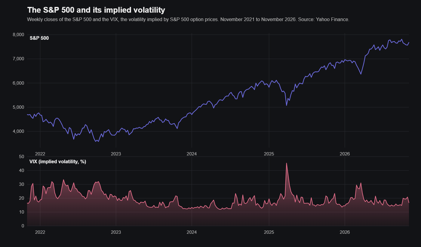
The second use is as a reading of sentiment. When implied volatility rises, the market is paying more for options, which usually means more uncertainty about where the price is going. When it falls, people are expecting a quieter period. The VIX is nothing more than this idea applied to the S&P 500.
The third is trading volatility itself. Some strategies, straddles and strangles being the best known, are not really bets on direction at all. They are bets that the realised movement will be larger or smaller than what the implied volatility is pricing in. You cannot run those without this calculation.
And the fourth is risk. If the implied volatility of an asset is 40 per cent annualised, you can translate that into an expected range over any period you like, and that range is a reasonable starting point for how much a position might move against you.
In the next post I take a real 30-day Bitcoin option and do the calculation in Python, with the actual numbers, because the explanation above only really lands once you have seen it produce a figure.