
I am going to write a series of posts about volatility, because it is the subject that comes up most when people ask me about trading and because it is the one I think is worst explained. This first one is the groundwork: what the word means, where volatility comes from, what it does to a trade, and the handful of things I actually do about it. The later posts get into the calculations.
All of this can be checked against every trading day of the S&P 500 since 1990, which is what the later sections do.
What it is
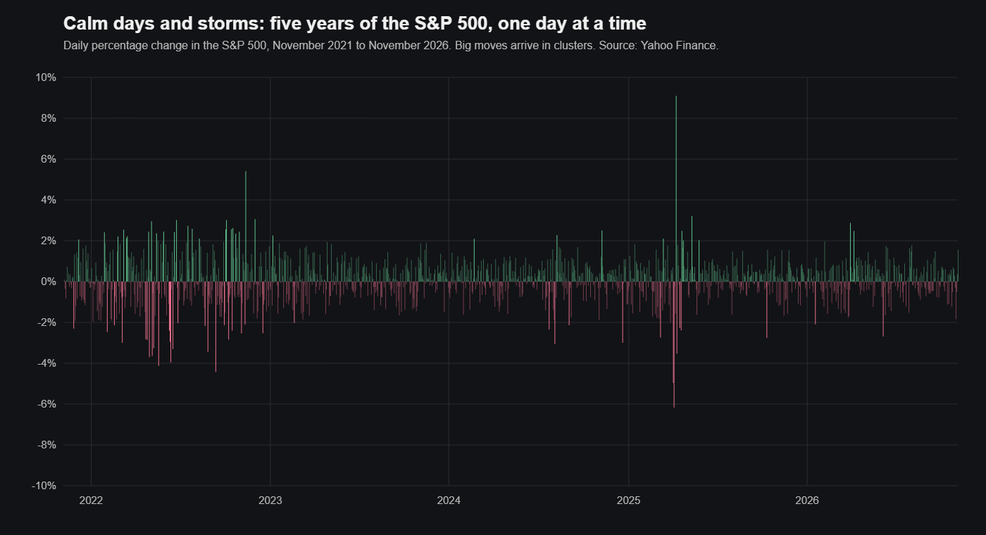
Volatility is a measure of how much the price of something moves over a given period. A market where prices drift within a narrow range has low volatility. A market where prices swing several per cent in a day has high volatility. When people put a number on it, that number is almost always the standard deviation of returns over some window, scaled to a year, which is why you see figures like “20 per cent volatility” for an equity index or “50 per cent” for Bitcoin. I will go through exactly how that number is built in a later post. For now the thing to hold on to is that volatility is about the size of the moves, not their direction. A market that is falling steadily can have low volatility. A market that is going nowhere but swinging wildly on the way has high volatility.
Why it matters
Every trade is a bet about direction, but the size of what you can win or lose on that bet is set by volatility. In a quiet market a wrong call costs you a little. In a volatile one the same wrong call can cost a great deal in a very short time, and a right call can pay out just as quickly. So volatility is where both the opportunity and the risk come from, and most of the discipline in trading is about keeping the second from eating the first.
It also changes the mechanics of trading in ways that are easy to forget until they cost you. In volatile markets the gap between the buying price and the selling price widens, so every trade is more expensive to put on and take off. Prices reverse quickly, so a position that looked right an hour ago can look wrong before you have finished deciding what to do about it. And it does something to people. Fear and greed are both stronger when the numbers on the screen are moving fast, and a trader who is usually disciplined can become impulsive in an afternoon. The only defence against that I know of is to have decided in advance what you will do, and then to do it.
Where it comes from
Volatility is not random noise. It usually has a source, and knowing the source tells you something about how long it will last.
Scheduled economic data is the most predictable one. Inflation figures, employment numbers, growth data and central bank decisions all have release dates, and the market moves when they come out because positions get adjusted all at once. Earnings releases do the same thing for individual stocks, with the move depending on how far the result is from what was expected. Geopolitical events, elections, wars and trade disputes, are the unscheduled version, and they tend to produce longer periods of elevated volatility because the uncertainty does not resolve on a single day.
Then there is sentiment, which is really the sum of everyone’s reaction to everything above. When people are frightened, selling begets selling and prices fall quickly; when they are overconfident, the reverse. And underneath all of it is liquidity. A thinly traded market or stock will move a long way on a small amount of buying or selling, simply because there is nobody on the other side, and that shows up as volatility whether or not anything has actually happened.
What thirty-six years of the S&P 500 show
Over 9,281 trading days from January 1990 to November 2026, the index’s volatility averaged 18.0% a year (on the price index, without dividends). Calendar years ranged from 6.7% in 2017 to 41.0% in 2008, and 2026 so far has run at 13.8%. It is the same index throughout. What changed from year to year was the regime.
The more useful finding is that volatility clusters. On 6.5% of days the index moved by more than 2% in either direction. On the day after such a move, the chance of another was 21.0%, more than three times as high. The size of a day’s move is correlated with the size of the moves before it, 0.27 a day apart, 0.20 a month apart and still 0.12 three months apart, while the direction has almost no memory: −0.08 a day apart and close to zero after that. That is the statistical version of the section above: volatility has a source, and it lasts. It is also why sizing to recent volatility works at all. If quiet and violent days arrived at random, yesterday’s volatility would say nothing about tomorrow’s.
What I actually do about it
None of this is exotic, and most of it is about sizing rather than cleverness.
I size positions to the volatility, not to a fixed amount of money. If an asset’s volatility doubles, I halve the position, so that the amount I can lose on a normal bad day stays roughly constant. There is a mathematical way to do this properly, which I will come to in a later post, but even the rough version is better than ignoring it.
I use stops, and I set them wide enough that ordinary noise does not trigger them. A stop that sits inside the range of a normal day’s movement is not protection, it is a way of being taken out of a position at the worst moment. The width of a normal day is exactly what volatility tells you, which is why the two decisions go together.
I keep leverage low when volatility is high. Leverage multiplies both gains and losses, and in a volatile market the losses arrive before you have time to react to them.
I spread exposure across things that do not move together, which is the whole point of diversification and is harder to achieve than it sounds, because in a sell-off most things start moving together. I have a separate post on that under correlation.
I watch volatility as a quantity in its own right. The average true range, which I will show how to calculate, is a simple way of tracking whether an asset’s daily movement is growing or shrinking, and a rising reading is often the first sign that the regime is changing.
And occasionally I trade it directly. Options and volatility products let you take a position on whether the coming moves will be bigger or smaller than the market is currently pricing, independent of direction. That is a more advanced subject and needs its own posts, but it is worth knowing it exists, because once you see volatility as something with a price, a lot of the rest of trading makes more sense.
The next post in the series looks at the two kinds of volatility you will hear about most, historical and implied, and why the gap between them matters.
Sizing to volatility, tested
The first habit on that list is easy to test. Each day, hold the S&P 500 in a size equal to a target volatility divided by the index’s volatility over the previous 21 trading days, capped at twice the capital, so that a doubling of volatility halves the position. Then compare it with holding the index at a fixed size, from the end of January 1990 to November 2026, with no trading costs and no interest on cash or borrowing.
| Return a year | Volatility | Worst fall | Worst day | 12-month range | |
|---|---|---|---|---|---|
| Fixed size | 8.9% | 18.0% | −56.8% | −12.0% | 6.7% to 45.6% |
| Sized to 10% volatility | 6.7% | 11.0% | −36.0% | −5.6% | 9.7% to 13.0% |
| Sized to 15% volatility | 9.4% | 16.2% | −49.5% | −6.9% | 13.0% to 19.0% |
Price index without dividends, so all three returns sit roughly two percentage points a year below what a holder of the index actually earned.
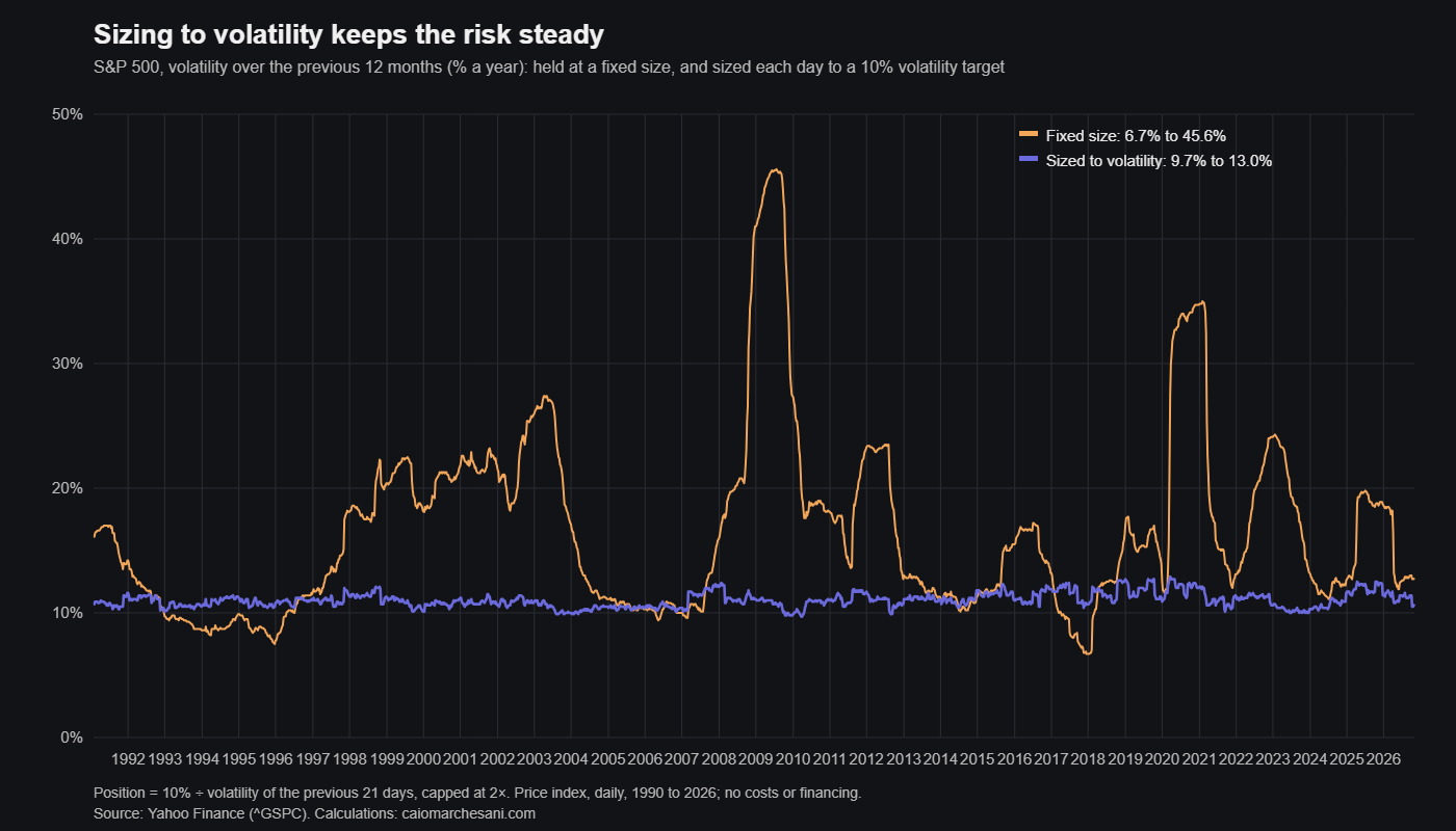
The sized versions do what the rule promises. Their volatility over any twelve months stayed within a few points of the target, against a range of 6.7% to 45.6% for the fixed position, and the worst single day was roughly half as bad. Return per unit of risk improved from 0.49 to 0.60 for the 10% version and 0.58 for the 15% version. The 15% version also made more than the index, but that came from borrowing in calm markets, with an average position of 1.2 times capital, and the cost of that borrowing is not in these numbers.
It does not remove drawdowns. A 21-day measure reacts to a crash only after its first days, so the sized versions still fell 36% and 50% at their worst. What it changes is how much of the damage arrives in a single day and how widely the risk of the book swings from one year to the next, which is the part a trader can control.
Checking it yourself
Everything quoted above can be reproduced with this script. It needs pandas and yfinance, and it starts from the S&P 500’s daily closes back to the start of 1990.
import numpy as np
import pandas as pd
import yfinance as yf

px = yf.download("^GSPC", start="1989-12-01", end="2026-11-07",
                 auto_adjust=False, progress=False)["Close"].squeeze()
r = np.log(px).diff().dropna().loc["1990-01-02":]

yearly = r.groupby(r.index.year).std() * np.sqrt(252) * 100
print(f"Volatility {r.std() * np.sqrt(252):.1%} a year;",
      f"calmest year {yearly.idxmin()} ({yearly.min():.1f}%),",
      f"wildest {yearly.idxmax()} ({yearly.max():.1f}%)")

big = r.abs() > 0.02
print(f"Days with a move above 2%: {big.mean():.1%};",
      f"the day after one: {big[big.shift(1, fill_value=False)].mean():.1%}")


def acf(x, k):
    x = x - x.mean()
    return (x.values[k:] * x.values[:-k]).sum() / (x.values ** 2).sum()


print("Autocorrelation, size of move:",
      " ".join(f"{k}d {acf(r.abs(), k):.2f}" for k in (1, 5, 21, 63, 252)))
print("Autocorrelation, direction:   ",
      " ".join(f"{k}d {acf(r, k):+.2f}" for k in (1, 5, 21)))


def stats(daily):
    equity = (1 + daily).cumprod()
    log = np.log(1 + daily)
    years = len(daily) / 252
    roll = log.rolling(252).std().dropna() * np.sqrt(252)
    cagr = equity.iloc[-1] ** (1 / years) - 1
    vol = log.std() * np.sqrt(252)
    drawdown = (equity / equity.cummax() - 1).min()
    return (f"{cagr:6.1%} {vol:6.1%} {drawdown:7.1%} {daily.min():6.1%}"
            f"   {roll.min():.1%} to {roll.max():.1%}")


sigma = r.rolling(21).std().shift(1) * np.sqrt(252)
simple = np.exp(r) - 1
keep = sigma.notna()
print("                       return    vol drawdown  worst   1-year vol")
print("Buy and hold          ", stats(simple[keep]))
for target in (0.10, 0.15):
    weight = (target / sigma).clip(upper=2)
    print(f"Sized to {target:.0%} vol      ", stats((weight * simple)[keep]))
Run in November 2026 it prints:
Volatility 18.0% a year; calmest year 2017 (6.7%), wildest 2008 (41.0%)
Days with a move above 2%: 6.5%; the day after one: 21.0%
Autocorrelation, size of move: 1d 0.27 5d 0.32 21d 0.20 63d 0.12 252d 0.03
Autocorrelation, direction:    1d -0.08 5d -0.02 21d -0.01
                       return    vol drawdown  worst   1-year vol
Buy and hold             8.9%  18.0%  -56.8% -12.0%   6.7% to 45.6%
Sized to 10% vol         6.7%  11.0%  -36.0%  -5.6%   9.7% to 13.0%
Sized to 15% vol         9.4%  16.2%  -49.5%  -6.9%   13.0% to 19.0%