
On the first trading day of 2022, the standard textbook risk model put a 60/40 portfolio’s worst day in a hundred at a loss of 1.15%. The portfolio went on to lose more than that on 17 days that year.
You’d expect two or three. I wanted to know whether 2022 was a freak, or whether the model had been wrong for a long time without anyone much noticing, and if so which part of it was wrong. So I rebuilt the portfolio from daily ETF prices going back to 2002 and ran three common value-at-risk models over it, then put each one through the two backtests that risk teams and regulators rely on. It all runs from one Python script, which is at the bottom.
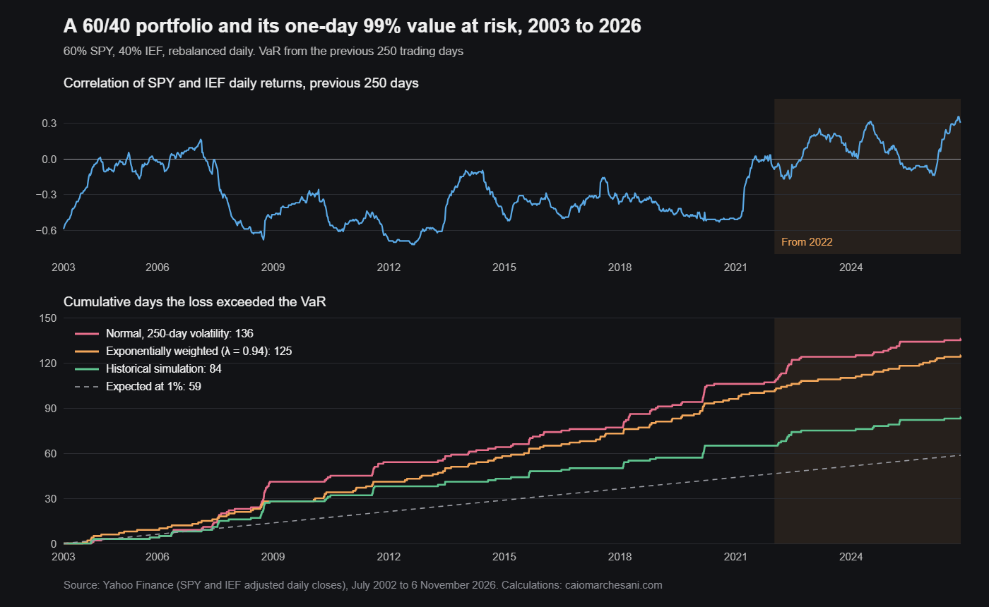
The portfolio and the three models
The portfolio is 60% SPY, the S&P 500 ETF, and 40% IEF, which holds 7 to 10 year US Treasuries. I rebalance it every day and use Yahoo Finance’s adjusted closes, so dividends and coupons are in the returns. IEF only started trading at the end of July 2002 and each model needs 250 trading days behind it, which makes 29 July 2003 the first day with a forecast. That leaves 5,858 days to test.
All three models produce a one-day 99% VaR: the loss the portfolio should exceed on only about one trading day in a hundred. None of them sees anything later than the previous close.
Every textbook has the first one. Take the standard deviation of the last 250 daily portfolio returns and multiply by 2.326, the point on a normal curve that leaves 1% below it. With two assets you can write that standard deviation out in full:
\[\sigma_p = \sqrt{w_1^2\sigma_1^2 + w_2^2\sigma_2^2 + 2\,w_1 w_2\,\rho\,\sigma_1\sigma_2}\]The hedge is all in the last term. When stocks and bonds move against each other ρ is negative, and the portfolio is less risky than its two legs added up. The model reads ρ off the last 250 days and assumes tomorrow will look the same.
Historical simulation doesn’t assume a shape at all. It sorts those 250 returns and reads off the 1% point, which sits between the third and fourth worst days.
The third model, the one RiskMetrics made popular in the 1990s, gives recent days more weight by updating the variance each day:
\[\sigma_t^2 = \lambda\,\sigma_{t-1}^2 + (1-\lambda)\,r_{t-1}^2, \qquad \lambda = 0.94\]At λ = 0.94 yesterday’s return gets 6% of the weight, and any one day’s influence halves in about eleven trading days. In pandas the three models are a few lines. The shift(1) is what stops each forecast from seeing its own day:
var = pd.DataFrame({
    "normal": -Z * port.rolling(W).std().shift(1),
    "historical": port.rolling(W).quantile(0.01).shift(1),
    "EWMA": ewma_var(port),
}).dropna()
If the portfolio loses more than that morning’s VaR, the day is an exception.
All three fail the count, and two fail the timing
There are two standard tests, and they ask different things. Kupiec’s is about the count: is the number of exceptions believable for a model that promised 1%? It compares how likely the observed breaches were at that 1% rate with how likely they were at the rate that actually turned up. Christoffersen’s is about timing. It checks whether a breach is more likely the day after another breach, which is what clustering looks like. Either statistic above 3.84, the 5% critical value of chi-squared with one degree of freedom, is a fail. Both are set out step by step in my longer piece on value at risk.
| Model | Exceptions | Share of days | Kupiec | Christoffersen | Back-to-back |
|---|---|---|---|---|---|
| Normal, 250 days | 136 | 2.32% | 75.3 | 28.8 | 16 |
| Historical simulation | 84 | 1.43% | 9.8 | 26.7 | 10 |
| EWMA, λ = 0.94 | 125 | 2.13% | 57.4 | 3.2 | 6 |
5,858 trading days from 29 July 2003 to 6 November 2026, SPY and IEF adjusted closes from Yahoo Finance. A model that was right would expect about 59 exceptions. Back-to-back counts pairs of consecutive days that were both exceptions.
The normal model was breached 136 times, more than double what it promised. Historical simulation got closest, at 1.43%, and still fails Kupiec. Both fail Christoffersen badly. Their breaches come in runs, because a 250-day window moves so slowly that after one bad week it stays out of date for several more.
EWMA is the odd one. It’s breached almost as often as the normal model, yet the breaches are spread out and it passes the clustering test at 3.2. My reading is that it forgets as fast as it learns: a quiet fortnight drags its VaR down, and then fairly ordinary days go through it.
The lower panel of the chart shows how the breaches arrive. They bunch up in the bad years. Here are four of those years:
| Exceptions in | 2008 | 2018 | 2020 | 2022 |
|---|---|---|---|---|
| Normal, 250 days | 19 | 14 | 12 | 17 |
| Historical simulation | 12 | 7 | 8 | 10 |
| EWMA, λ = 0.94 | 8 | 8 | 10 | 7 |
A model keeping its promise would be breached two or three times in a year.
In 2022 the volatility did more damage than the correlation
2022 usually gets told as the year the stock and bond hedge died, and the correlation did flip sign. SPY returned −18.2% with dividends and IEF −15.2%, so the 60/40 lost 16.4%. Its worst day was 13 June, down 2.99%.
The normal model’s own inputs let you split the damage. Going into 2022, the previous 250 days gave a daily standard deviation of 0.82% for SPY and 0.34% for IEF with a correlation of −0.08, and that is where the 1.15% VaR came from. During 2022 the standard deviations were 1.53% and 0.64% and the correlation was +0.19. Put the 2022 volatilities into the formula but keep the old correlation, and the VaR comes out at 2.16%. Swap in the 2022 correlation as well and it’s 2.32%.
So the model was short by 1.17 points, and roughly 1.01 of that was volatility nearly doubling. The correlation accounts for 0.16. That isn’t the split the usual story implies. Part of the explanation is that the correlation in the window was already up at −0.08 by the end of 2021, against an average of −0.34 over 2003 to 2021. A good deal of the hedge had gone before the year began, and the model knew it.
Where the correlation does show up is in what the bad days looked like. Before 2022, SPY and IEF fell on the same day 15.2% of the time. In 2022 they did so on 33.5% of days, and 12 of the normal model’s 17 exceptions were days like that.
And it hasn’t gone back. To the end of 2021 the 250-day correlation was below zero on 92.8% of days. Since the start of 2022 that’s 35.1%, the average is +0.07, and the latest reading is +0.28. I went through the same shift for stocks and Treasury futures in a longer piece on correlation in trading.
Changes I would make to a model like this
Backtesting by regime, as well as in total, comes first. A model fitted on 2003 to 2021 carried a hedge that has been missing more often than not since then. Split the backtest at 2022 and you see it straight away, where the full-sample totals bury it.
I’d also never report the exception rate without the clustering test next to it. On the count alone historical simulation looks best, and on clustering it looks worst, with EWMA the other way round. If your problem is a bad week more than a bad day, the count ranks them the wrong way.
There’s a cheap early warning in the share of days when both legs fall together. It needs no model, and in 2022 it more than doubled, from 15.2% to 33.5%.
Lastly, I’d stress volatility at least as hard as correlation. In this sample a correlation shock by itself would have moved the VaR much less than the doubling of volatility did.
The setup is deliberately simple, and it has limits. Daily rebalancing is one of them: a book rebalanced monthly drifts towards whichever leg has done better, and its risk drifts with it. ETF prices carry small tracking differences against the indices they follow. And passing a 99% VaR test tells you nothing about how bad the days beyond it are. For that you need expected shortfall, which has to be backtested separately.
Checking it yourself
The script downloads both ETFs with yfinance, builds the portfolio, runs the three models and the two tests, and prints every number I’ve quoted. You need numpy, pandas and yfinance, nothing else.
import numpy as np
import pandas as pd
import yfinance as yf

px = yf.download(["SPY", "IEF"], start="2002-07-01", end="2026-11-07",
                 auto_adjust=True, progress=False)["Close"].dropna()
r = px.pct_change().dropna()
port = 0.6 * r["SPY"] + 0.4 * r["IEF"]          # rebalanced to 60/40 every day
W, Z, LAM = 250, 2.3263478740408408, 0.94      # window, 99% normal quantile, RiskMetrics decay


def ewma_var(x):
    out = pd.Series(np.nan, index=x.index)
    v = (x.iloc[:W] ** 2).mean()
    for i in range(W, len(x)):
        if i > W:
            v = LAM * v + (1 - LAM) * x.iloc[i - 1] ** 2
        out.iloc[i] = -Z * np.sqrt(v)
    return out


var = pd.DataFrame({
    "normal": -Z * port.rolling(W).std().shift(1),
    "historical": port.rolling(W).quantile(0.01).shift(1),
    "EWMA": ewma_var(port),
}).dropna()
ret = port.loc[var.index]


def kupiec(hit, p=0.01):
    T, x = len(hit), hit.sum()
    q = x / T
    return -2 * ((T - x) * np.log(1 - p) + x * np.log(p) - (T - x) * np.log(1 - q) - x * np.log(q))


def christoffersen(hit):
    a, b = hit[:-1], hit[1:]
    n = {(i, j): int(((a == i) & (b == j)).sum()) for i in (0, 1) for j in (0, 1)}
    p01 = n[0, 1] / (n[0, 0] + n[0, 1])
    p11 = n[1, 1] / (n[1, 0] + n[1, 1])
    p = (n[0, 1] + n[1, 1]) / sum(n.values())
    ll = lambda k, q: k * np.log(q) if k else 0.0
    return -2 * (ll(n[0, 0] + n[1, 0], 1 - p) + ll(n[0, 1] + n[1, 1], p)
                 - ll(n[0, 0], 1 - p01) - ll(n[0, 1], p01) - ll(n[1, 0], 1 - p11) - ll(n[1, 1], p11)), n[1, 1]


print(f"60/40 SPY/IEF, {len(ret)} days of one-day 99% VaR, {ret.index[0]:%d %b %Y} to {ret.index[-1]:%d %b %Y}")
print("method      exceptions  share  Kupiec  Christoffersen  back-to-back  2008  2018  2020  2022")
for m in var:
    hit = (ret < var[m]).astype(int).to_numpy()
    lr_ind, n11 = christoffersen(hit)
    by_year = pd.Series(hit, index=ret.index).groupby(ret.index.year).sum()
    print(f"{m:<11}{hit.sum():>10}{hit.mean():>7.2%}{kupiec(hit):>8.1f}{lr_ind:>16.1f}{n11:>14}"
          + "".join(f"{by_year.get(y, 0):>6}" for y in (2008, 2018, 2020, 2022)))

end21, y22 = r.loc[:"2021-12-31"].iloc[-W:], r.loc["2022"]
sd = lambda w, rho: Z * np.sqrt(0.36 * w[0] ** 2 + 0.16 * w[1] ** 2 + 0.48 * rho * w[0] * w[1])
s21, s22 = end21.std().to_numpy(), y22.std().to_numpy()
c21, c22 = end21.corr().iloc[0, 1], y22.corr().iloc[0, 1]
print(f"\n2022: SPY {(1 + y22['SPY']).prod() - 1:.1%}, IEF {(1 + y22['IEF']).prod() - 1:.1%}, "
      f"60/40 {(1 + port.loc['2022']).prod() - 1:.1%}; worst day {port.loc['2022'].min():.2%} "
      f"on {port.loc['2022'].idxmin():%d %b}")
print(f"  daily sd SPY {s21[0]:.2%} -> {s22[0]:.2%}, IEF {s21[1]:.2%} -> {s22[1]:.2%}; "
      f"correlation {c21:.2f} -> {c22:.2f}")
print(f"  normal VaR on 3 Jan 2022 {sd(s21, c21):.2%}; with 2022 volatility {sd(s22, c21):.2%}; "
      f"with 2022 volatility and correlation {sd(s22, c22):.2%}")
hit22 = ret.loc["2022"] < var["normal"].loc["2022"]
both = (r["SPY"] < 0) & (r["IEF"] < 0)
print(f"  normal-VaR exceptions in 2022 on days both fell: {(hit22 & both.loc[hit22.index]).sum()} of {hit22.sum()}; "
      f"days both fell: {both.loc['2022'].mean():.1%} of 2022, {both.loc[var.index[0]:'2021'].mean():.1%} before")

rho = r["SPY"].rolling(W).corr(r["IEF"]).shift(1).loc[var.index]
print(f"\n250-day SPY/IEF correlation: negative on {(rho.loc[:'2021'] < 0).mean():.1%} of days to 2021 "
      f"(average {rho.loc[:'2021'].mean():.2f}), {(rho.loc['2022':] < 0).mean():.1%} since "
      f"(average {rho.loc['2022':].mean():.2f}); latest {rho.iloc[-1]:.2f}")
This is what it printed on 11 November 2026, with prices up to 6 November:
60/40 SPY/IEF, 5858 days of one-day 99% VaR, 29 Jul 2003 to 06 Nov 2026
method      exceptions  share  Kupiec  Christoffersen  back-to-back  2008  2018  2020  2022
normal            136  2.32%    75.3            28.8            16    19    14    12    17
historical         84  1.43%     9.8            26.7            10    12     7     8    10
EWMA              125  2.13%    57.4             3.2             6     8     8    10     7

2022: SPY -18.2%, IEF -15.2%, 60/40 -16.4%; worst day -2.99% on 13 Jun
  daily sd SPY 0.82% -> 1.53%, IEF 0.34% -> 0.64%; correlation -0.08 -> 0.19
  normal VaR on 3 Jan 2022 1.15%; with 2022 volatility 2.16%; with 2022 volatility and correlation 2.32%
  normal-VaR exceptions in 2022 on days both fell: 12 of 17; days both fell: 33.5% of 2022, 15.2% before

250-day SPY/IEF correlation: negative on 92.8% of days to 2021 (average -0.34), 35.1% since (average 0.07); latest 0.28
Yahoo recalculates adjusted prices now and then, so if you run it later the last digit may differ.