
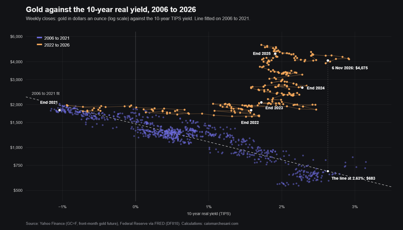
On the line that priced gold for sixteen years, an ounce should cost about $680 today. On 6 November 2026 it closed at $4,075.
The line is the standard macro model of gold: the price against the real yield on ten-year US Treasuries. From 2006 to 2021 it explained most of what gold did. I rebuilt it on twenty years of weekly data to see when it stopped working, by how much, and whether any part of it is still worth using.
Why gold should care about real yields
Gold pays no interest. A ten-year inflation-protected Treasury, a TIPS, pays a yield on top of inflation, and that is the real yield. So the real yield is what you give up by holding gold instead of the safest inflation-proof asset there is.
When the real yield is 2 per cent, gold has to beat inflation by 2 per cent a year just to keep up. When it is minus 1 per cent, as it was in 2021, the bond is guaranteed to lose purchasing power and gold only has to hold its value. Low real yields, high gold. That was the whole model.
Sixteen years on one line
I took Friday closes of the front-month gold future and the ten-year TIPS yield from January 2006 to December 2021, 835 weeks, and fitted the logarithm of the gold price to the real yield.
\[\text{gold} \approx 1{,}465 \times e^{-0.29\,r}\]Gold is in dollars an ounce and r is the real yield in percentage points. The line puts gold at $1,465 when the real yield is zero and takes about 25 per cent off for every point the real yield rises. Over those sixteen years it explained 85 per cent of the variation in the price, and its typical miss was 12 per cent.
At the end of 2021 the real yield was −1.04 per cent. The line said $1,981. Gold was at $1,829. That is about as well as a one-variable model ever works.
One caution. A regression of one slow-moving series on another flatters itself, and an R² of 85 per cent can come from two trends that have nothing to do with each other. The test that separates a real relationship from a coincidence of trends is cointegration: if the two series are tied together, the gap between gold and the line should keep closing, and it should be possible to say how fast.
Call the gap e, the logarithm of gold minus the logarithm of the line, and fit the standard Engle and Granger test, an augmented Dickey and Fuller regression on the gap:
\[\Delta e_t = \alpha + \gamma\, e_{t-1} + \phi\, \Delta e_{t-1} + \varepsilon_t\]If γ is negative and clearly different from zero, the gap is pulled back towards nothing. On 2006 to 2021 the t-statistic on γ is −4.31, against a 5 per cent critical value of −3.34 for a two-variable test. Gold and the real yield were cointegrated. The speed of the pull gives a half-life:
\[\text{half-life} = \frac{\ln 0.5}{\ln(1+\gamma)}\]It comes out at 16 weeks. When gold strayed from the line it closed half the distance in about four months, and in sixteen years it was never more than 38 per cent above it. That is what made it a model a trader could use, and not just a correlation on a chart.
Real yields rose 3.6 points and gold did not fall
Then real yields turned. Between the last week of July 2021 and the first week of October 2023 the ten-year real yield went from −1.16 per cent to 2.47 per cent. On the line, that should have cut the gold price by 65 per cent. Gold went from $1,813 to $1,845. It rose 2 per cent.
Take 2022 on its own. The real yield rose 2.6 points over the year, and the line fell by more than half, from $1,981 to $926. Gold ended the year at $1,826, three dollars from where it began.
The gap has widened every year since.
| Week ending | Real yield | Gold | The line | Gold ÷ line |
|---|---|---|---|---|
| 31 Dec 2021 | −1.04% | $1,829 | $1,981 | 0.92 |
| 30 Dec 2022 | 1.58% | $1,826 | $926 | 1.97 |
| 29 Dec 2023 | 1.72% | $2,072 | $889 | 2.33 |
| 27 Dec 2024 | 2.28% | $2,632 | $756 | 3.48 |
| 26 Dec 2025 | 1.91% | $4,553 | $841 | 5.41 |
| 6 Nov 2026 | 2.63% | $4,075 | $683 | 5.97 |
Friday closes. Gold is the front-month COMEX future, from Yahoo Finance. The real yield is the ten-year TIPS yield, from the Federal Reserve through FRED. “The line” is the 2006 to 2021 fit applied to that week’s real yield.
A miss of 12 per cent is normal for a model like this. A miss of six times means something else is setting the price.
Dating the break
The timing matters for the explanation, so I measured it. The second chart divides gold by the line, week by week. The shaded band is two typical misses either side, about 24 per cent, which gold stayed inside for 787 of the 835 weeks from 2006 to 2021. The exceptions were early 2006, below it, and the run-up to the 2011 peak, above it.
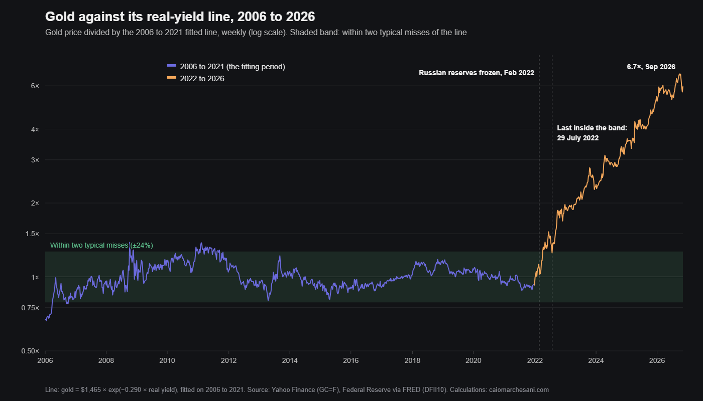
At the end of February 2022 gold was 9 per cent above the line, well inside the band. It left the band for good after 29 July 2022 and has been above it every week since. It passed twice the line in May 2023 and reached 6.7 times it in September 2026.
The cointegration test confirms it. Refit the line on the whole of 2006 to 2026 and run the same regression on the gap: the t-statistic is −0.18, nowhere near the critical value, and the implied half-life is 2,360 weeks. In plain terms, the gap no longer closes. The relationship did not get noisier. It stopped being an equilibrium.
A buyer who does not look at yields
The explanation I find most convincing is who was buying. In February 2022 the United States and its allies froze the Russian central bank’s reserves held in their currencies. For any central bank that could picture itself on the wrong side of a sanctions list, gold held at home became the one reserve asset nobody else can switch off.
The World Gold Council’s figures show what followed. Central banks bought more than 1,000 tonnes of gold in each of 2022, 2023 and 2024, and 863 tonnes in 2025. The average from 2010 to 2021 was 473 tonnes a year.
A reserve manager making that decision is not comparing gold with a TIPS yield. The old model assumed that the buyer who set the price was an investor choosing between the two. From 2022 a large share of the buying came from someone asking a different question, and the price stopped answering to the real yield.
The flows show the mechanism more precisely than the totals do. Gold held through exchange-traded funds sits mostly in North American and European funds, and its owners are exactly the investors the real-yield model describes. Here is what they did, next to the central banks.
| Year | Real yield, year end | Gold, year end | Central banks | Gold ETFs |
|---|---|---|---|---|
| 2022 | 1.58% | $1,826 | +1,082 t | −110 t |
| 2023 | 1.72% | $2,072 | +1,037 t | −244 t |
| 2024 | 2.28% | $2,632 | +1,092 t | −3 t |
| 2025 | 1.91% | $4,553 | +863 t | +801 t |
Net purchases in tonnes, from the World Gold Council’s full-year reports for 2023 (2022 and 2023) and 2025 (2024 and 2025); the Council revises earlier years. Prices and yields as in the first table.
The ETF holders behaved exactly as the model said they would. Real yields rose by 2.6 points in 2022 and they sold 110 tonnes, then another 244 tonnes in 2023. On its own that selling should have pushed the price down towards the line. It did not, because over the same two years central banks bought 2,119 tonnes.
That is the technical point. A market price is set where the holders who are sensitive to price are willing to hold whatever the insensitive buyers leave them. The line described those sensitive holders, and their sensitivity, as far as the weekly numbers can measure it, changed far less than the level did. What changed is that a buyer who does not respond to price or yield started taking more than a thousand tonnes a year, so the sensitive holders had to be offered a higher price at every level of the real yield before they would give up the metal. In the model, that is not a change in the slope. It is a shift in the constant.
2025 is the year the second group stopped selling. ETFs bought 801 tonnes, central-bank buying slowed by about a fifth, and gold rose 73 per cent.
Other explanations are offered, and they are not rivals. Large deficits with no recession to excuse them, which I wrote about in the pandemic piece, give private investors their own reason to want an asset that is nobody’s liability. I cannot separate the two with a regression. What the data does show is the timing: the line held until the end of 2021 and was out by a factor of two within a year.
The weekly relationship survived
The level broke. The week-to-week relationship did not, or not entirely.
From 2006 to 2021 the correlation between the weekly change in the real yield and the weekly change in gold was −0.30, and a one-point rise in the real yield went with a fall of 6.9 per cent in gold. From 2022 to 2026 the figures are −0.24 and 4.9 per cent. Weaker, and still there. For comparison, the same weekly figure for Bitcoin is −0.09, which I measured in the piece on Bitcoin and the Fed.
The dollar is the obvious thing that could be confusing this, because a stronger dollar tends to push gold down and tends to rise with US real yields. So I put both in the same weekly regression. From 2006 to 2021 gold fell 4.0 per cent for a one-point rise in the real yield (t-statistic −5.6) and 1.31 per cent for a 1 per cent rise in the broad dollar index (t −13.0). From 2022 to 2026 the figures are 2.7 per cent (t −2.2) and 1.27 per cent (t −5.8).
The dollar effect is unchanged. The real-yield effect is about two-thirds of what it was and much less certain, but it has not gone. Put that next to the cointegration result and the picture is consistent: the week-to-week slope mostly survived, and the level it is measured from moved. That is what the flows above would predict.
Two other things stand out. The first is that the weekly sensitivity was always far smaller than the 25 per cent a point in the line. Most of that 25 per cent came from two series drifting in opposite directions for years, which is the flattery I mentioned above.
The second is 2025. Year by year from 2022, the weekly correlation was −0.31, −0.60, −0.23, +0.30 and −0.36. In 2025, the year gold went from $2,632 to $4,553, gold and real yields rose and fell together. Central-bank buying was down by a fifth that year, and investment demand was up 84 per cent, to 2,175 tonnes. When investors are chasing a price, even the short-run link can go.
Over a rolling 52 weeks the correlation was below zero in 753 of 783 weeks up to 2021, and in 202 of 253 since.
What is left of the model
I no longer use the level. A fair-value line at $683 tells me nothing about a market trading at $4,075, and waiting for the two to meet would have been wrong in every year since 2022.
I still use the direction. In most weeks a rise in real yields is a headwind for gold, about 5 per cent for a full point on the recent numbers. That has held in 2026: the real yield went from 1.91 per cent at the end of 2025 to 2.63 per cent in early November, and gold fell from $4,553 to $4,075.
And I watch the buyer. If central-bank purchases fall back towards the 473 tonnes a year of the previous decade, the old line starts to matter again, and the distance to it is large. If they do not, the line stays what it is now, a record of how the market used to work.
The honest way to rebuild the model would be to let the constant move with official buying, so that the line shifts up as central banks accumulate. I have not done it, because quarterly tonnages give about twenty observations since 2022, and a regression on twenty points with a trend in both series would flatter itself in exactly the way the original line did.
The stock and bond correlation changed sign in the same year, which I went through in the piece on correlation. Both make the same point: a relationship measured in one regime says little about the next one.
Checking it yourself
The price, yield and dollar figures above come from the script below, including both cointegration tests and the date of the break. It needs pandas, numpy and yfinance, and reads the TIPS yield and the broad dollar index straight from FRED. The tonnages are the World Gold Council’s.
import numpy as np
import pandas as pd
import yfinance as yf

FRED = "https://fred.stlouisfed.org/graph/fredgraph.csv?id="


def fred(series):
    return pd.read_csv(FRED + series, index_col=0, parse_dates=True,
                       na_values=".").squeeze()


def ols(y, *x):
    """Coefficients (constant first), t-statistics and R-squared."""
    X = np.column_stack([np.ones(len(y))] + [np.asarray(v, float) for v in x])
    y = np.asarray(y, float)
    b = np.linalg.solve(X.T @ X, X.T @ y)
    e = y - X @ b
    t = b / np.sqrt(e @ e / (len(y) - X.shape[1]) * np.diag(np.linalg.inv(X.T @ X)))
    return b, t, 1 - (e @ e) / ((y - y.mean()) @ (y - y.mean()))


def adf(e):
    """Engle-Granger step two: ADF with a constant and one lag. t and half-life."""
    e = np.asarray(e, float)
    d = np.diff(e)
    b, t, _ = ols(d[1:], e[1:-1], d[:-1])
    return t[1], np.log(0.5) / np.log(1 + b[1])


gold = yf.download("GC=F", start="2006-01-01", end="2026-11-07",
                   progress=False)["Close"].squeeze()
real = fred("DFII10")                          # 10-year TIPS yield, per cent
usd = fred("DTWEXBGS")                         # broad trade-weighted dollar

w = pd.DataFrame({"gold": gold, "real": real}).dropna()
w = w.resample("W-FRI").last().dropna()        # Friday closes
old = w.loc[:"2021"]

b, _, r2 = ols(np.log(old.gold), old.real)
fit = np.exp(b[0] + b[1] * w.real)
gap = np.log(w.gold / fit)                     # log distance from the line
miss = gap.loc[:"2021"].std(ddof=2)
print(f"2006-2021 fit ({len(old)} weeks): gold = ${np.exp(b[0]):,.0f} x",
      f"exp({b[1]:.3f} x real yield), R2 {r2:.2f}")
print(f"  one point on the real yield: {np.exp(b[1]) - 1:+.0%} on gold;",
      f"typical miss {miss:.0%}")

stat, half = adf(gap.loc[:"2021"])
print(f"  cointegration test, 2006-2021: t = {stat:.2f}, half-life {half:.0f} weeks")
bw, _, _ = ols(np.log(w.gold), w.real)
stat, half = adf(np.log(w.gold) - bw[0] - bw[1] * w.real)
print(f"  same test, 2006-2026 refitted: t = {stat:.2f}, half-life {half:,.0f} weeks"
      " (5% critical value -3.34)")
inside = gap.index[gap <= 2 * miss][-1]
print(f"  last week within two typical misses of the line: {inside:%d %b %Y}")

print("Week ending  real yield     gold     fit  gold/fit")
for year in range(2021, 2027):
    row = w.loc[str(year)].iloc[-1]
    f = fit.loc[row.name]
    print(f"{row.name:%d %b %Y}  {row.real:10.2f}  {row.gold:7,.0f}  {f:6,.0f}"
          f"  {row.gold / f:8.2f}")

lo, hi = w.real.loc["2021"].idxmin(), w.real.loc["2023"].idxmax()
print(f"{lo:%d %b %Y} to {hi:%d %b %Y}: real yield {w.real[lo]:.2f} to"
      f" {w.real[hi]:.2f}, gold ${w.gold[lo]:,.0f} to ${w.gold[hi]:,.0f}"
      f" ({w.gold[hi] / w.gold[lo] - 1:+.0%}); the fit implied"
      f" {np.exp(b[1] * (w.real[hi] - w.real[lo])) - 1:+.0%}")

d = pd.DataFrame({"gold": np.log(w.gold).diff() * 100,
                  "real": w.real.diff()}).dropna()
for label, part in (("2006-2021", d.loc[:"2021"]), ("2022-2026", d.loc["2022":])):
    beta = ols(part.gold, part.real)[0][1]
    print(f"Weekly changes, {label}: correlation {part.gold.corr(part.real):+.2f},",
          f"{beta:+.1f}% on gold per point")
late = d.loc["2022":]
print("By year:", ", ".join(f"{year} {g.gold.corr(g.real):+.2f}"
                            for year, g in late.groupby(late.index.year)))
roll = d.gold.rolling(52).corr(d.real).dropna()
for label, part in (("to 2021", roll.loc[:"2021"]), ("since 2022", roll.loc["2022":])):
    print(f"52-week correlation {label}: below zero in {(part < 0).sum()} of"
          f" {len(part)} weeks, range {part.min():+.2f} to {part.max():+.2f}")

x = pd.DataFrame({"gold": gold, "real": real, "usd": usd}).dropna()
x = x.resample("W-FRI").last().dropna()
dx = pd.DataFrame({"gold": np.log(x.gold).diff() * 100, "real": x.real.diff(),
                   "usd": np.log(x.usd).diff() * 100}).dropna()
print("Weekly gold (%) on real yield (points) and the dollar (%), together:")
for label, p in (("2006-2021", dx.loc[:"2021"]), ("2022-2026", dx.loc["2022":])):
    bb, tt, rr = ols(p.gold, p.real, p.usd)
    print(f"  {label}: real yield {bb[1]:+.1f} (t {tt[1]:.1f}), dollar {bb[2]:+.2f}"
          f" (t {tt[2]:.1f}), R2 {rr:.2f}, {len(p)} weeks")
Run in November 2026 it prints:
2006-2021 fit (835 weeks): gold = $1,465 x exp(-0.290 x real yield), R2 0.85
  one point on the real yield: -25% on gold; typical miss 12%
  cointegration test, 2006-2021: t = -4.31, half-life 16 weeks
  same test, 2006-2026 refitted: t = -0.18, half-life 2,360 weeks (5% critical value -3.34)
  last week within two typical misses of the line: 29 Jul 2022
Week ending  real yield     gold     fit  gold/fit
31 Dec 2021       -1.04    1,829   1,981      0.92
30 Dec 2022        1.58    1,826     926      1.97
29 Dec 2023        1.72    2,072     889      2.33
27 Dec 2024        2.28    2,632     756      3.48
26 Dec 2025        1.91    4,553     841      5.41
06 Nov 2026        2.63    4,075     683      5.97
30 Jul 2021 to 06 Oct 2023: real yield -1.16 to 2.47, gold $1,813 to $1,845 (+2%); the fit implied -65%
Weekly changes, 2006-2021: correlation -0.30, -6.9% on gold per point
Weekly changes, 2022-2026: correlation -0.24, -4.9% on gold per point
By year: 2022 -0.31, 2023 -0.60, 2024 -0.23, 2025 +0.30, 2026 -0.36
52-week correlation to 2021: below zero in 753 of 783 weeks, range -0.81 to +0.07
52-week correlation since 2022: below zero in 202 of 253 weeks, range -0.62 to +0.30
Weekly gold (%) on real yield (points) and the dollar (%), together:
  2006-2021: real yield -4.0 (t -5.6), dollar -1.31 (t -13.0), R2 0.24, 834 weeks
  2022-2026: real yield -2.7 (t -2.2), dollar -1.27 (t -5.8), R2 0.16, 253 weeks