
On 21 February 2020 a standard one-day value at risk for the S&P 500 said that on ninety-nine days in a hundred the index would not fall by more than 1.7 per cent. Over the next twenty trading days it fell further than that eleven times.
Value at risk is the number most risk reports lead with, and the one regulators built capital rules on. I backtested the two simplest versions of it on 35 years of the S&P 500 and eleven of Bitcoin, then put them through the formal tests a regulator would use and tried a faster model against them, to see how often VaR is broken, by how much, when, and what can be done about it.
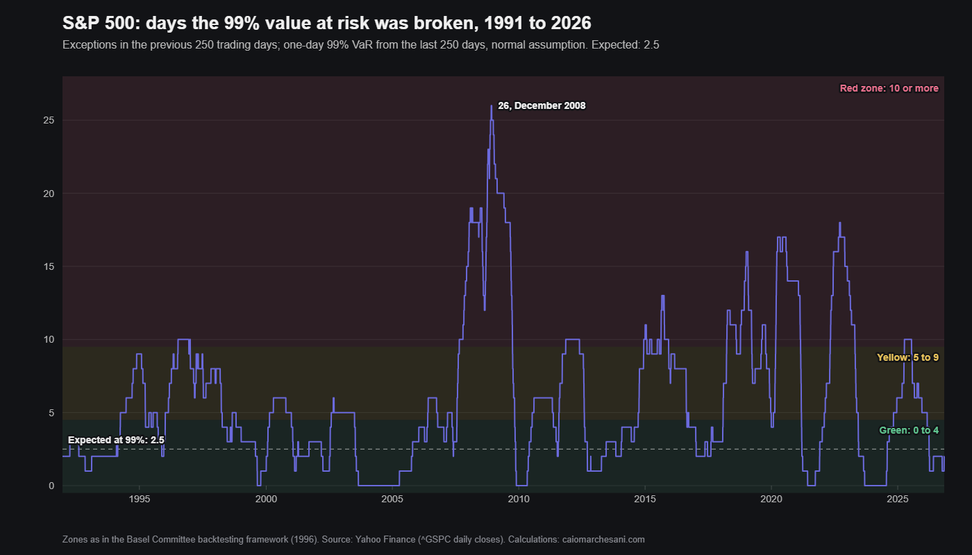
What the number says
A one-day 99 per cent VaR is a loss that should be exceeded on one day in a hundred. If it says $20,000 on a $1 million position, you expect to lose more than $20,000 on about two or three trading days a year. It says nothing about how much more. That gap matters, and I come back to it below.
The two versions I tested both look back over the last 250 trading days, about a year. The first assumes daily returns follow a normal distribution and scales their standard deviation by the point on the normal curve that leaves 1 per cent below it:
\[\text{VaR}_{99} = 2.326\,\sigma_{250}\]The second makes no assumption about the shape. It takes the 250 returns, sorts them and reads off the worst 1 per cent, which falls between the third and fourth worst day of the year. Both are recalculated each day using only data available the evening before, and each is compared with what happened the next day. A day when the loss is bigger than the VaR is called an exception.
Here is the calculation done by hand for the evening of 6 November 2026. Over the previous 250 trading days the S&P 500’s daily returns had a standard deviation of 0.856 per cent. Multiplied by 2.326 that gives a one-day 99 per cent VaR of 1.99 per cent, or about $19,700 on a $1 million position. The historical version sorts the same 250 days. The third and fourth worst were falls of 2.08 per cent and 1.83 per cent, and the 1 per cent point between them is 1.96 per cent, about $19,400. Two methods, almost the same answer, on a calm year.
The day before, 5 November 2026, the index had fallen 4.45 per cent, against a VaR of 1.89 per cent that morning. That was one of only two exceptions in the year, and it shows the problem in a single day: the VaR said what an ordinary bad day looks like, and the day that mattered was more than twice that.
Returns throughout are daily log returns in per cent. On an ordinary day the difference from the simple percentage change is negligible. On the worst days it is not, and I give both where it matters.
At 95 per cent it works; at 99 per cent it does not
| Market and VaR | Days | Exceptions | Share of days | Should be | Average loss ÷ VaR |
|---|---|---|---|---|---|
| S&P 500, 95%, normal | 9,031 | 469 | 5.2% | 5% | 1.54 |
| S&P 500, 95%, historical | 9,031 | 480 | 5.3% | 5% | 1.57 |
| S&P 500, 99%, normal | 9,031 | 208 | 2.3% | 1% | 1.42 |
| S&P 500, 99%, historical | 9,031 | 145 | 1.6% | 1% | 1.38 |
| Bitcoin, 95%, normal | 4,184 | 181 | 4.3% | 5% | 1.58 |
| Bitcoin, 95%, historical | 4,184 | 220 | 5.3% | 5% | 1.68 |
| Bitcoin, 99%, normal | 4,184 | 82 | 2.0% | 1% | 1.47 |
| Bitcoin, 99%, historical | 4,184 | 56 | 1.3% | 1% | 1.40 |
One-day VaR from the previous 250 days. S&P 500 from 27 December 1990, Bitcoin from 26 May 2015, both to 7 November 2026. Daily closes from Yahoo Finance.
At the 95 per cent level both versions are close enough on the S&P 500. At 99 per cent the normal version is broken on 2.3 per cent of days, more than twice as often as it claims. The historical version is better, at 1.6 per cent, and still too often.
Bitcoin shows the same thing more sharply. At 95 per cent the normal VaR is too cautious: it is broken on only 4.3 per cent of days. At 99 per cent it is broken twice as often as it should be. That is what fat tails look like in a backtest. Compared with a normal distribution of the same width, there are more quiet days and more violent ones, which I measured for 2021 in the piece on Bitcoin’s historical volatility. A model that fits the middle misses the edges.
Testing it properly
“Too often” needs a yardstick, because even a perfect model will not hit exactly 1 per cent in any sample. The standard test, Kupiec’s proportion-of-failures test, compares the likelihood of the exceptions you saw under the rate the model promised, p, with their likelihood under the rate you actually observed, x out of T days:
\[\text{LR}_{\text{POF}} = -2\ln\frac{(1-p)^{T-x}\,p^{x}}{(1-x/T)^{T-x}\,(x/T)^{x}}\]If the model is right, the statistic follows a chi-squared distribution with one degree of freedom, so anything above 3.84 rejects the model at the 5 per cent level. A second test, Christoffersen’s, asks a different question: is an exception more likely the day after another exception? It counts the four possible pairs of consecutive days (no exception then none, none then one, one then none, one then one) and uses the same 3.84 threshold. A model can pass one test and fail the other.
| 99% VaR | Share | Kupiec | Christoffersen | Again next day | Loss ÷ VaR |
|---|---|---|---|---|---|
| S&P 500, normal | 2.3% | 113.2 | 26.0 | 9% | 1.42 |
| S&P 500, historical | 1.6% | 28.3 | 21.4 | 8% | 1.38 |
| S&P 500, EWMA | 2.1% | 90.5 | 8.2 | 6% | 1.38 |
| Bitcoin, normal | 2.0% | 30.4 | 7.5 | 7% | 1.47 |
| Bitcoin, historical | 1.3% | 4.4 | 4.0 | 5% | 1.40 |
| Bitcoin, EWMA | 2.2% | 42.1 | 1.8 | 4% | 1.54 |
Kupiec and Christoffersen are likelihood-ratio statistics; above 3.84 the model is rejected at 5 per cent. “Again next day” is the share of exceptions followed by another exception the next trading day; if the model were right it would be 1 per cent. EWMA is the exponentially weighted model described further down.
Every version fails on the S&P 500, and by a wide margin. The historical VaR on Bitcoin comes closest to passing, at 4.4 and 4.0, which says the historical method copes with fat tails better than the normal one. The column I find most telling is the fifth. After a day that broke the S&P 500’s normal VaR, the next day broke it 9 per cent of the time. A model that is right would give 1 per cent. One exception is a warning that the next one is nine times more likely than the model thinks.
The loss when it is broken
The last column of the first table is the one I care about most. On a day when the S&P 500 broke its 99 per cent normal VaR, the loss averaged 1.42 times the VaR. If returns really were normal, it would be 1.15 times, which follows from the shape of the normal curve beyond 2.326 standard deviations.
So the model is wrong twice. It is broken more often than it says, and when it is broken the loss is bigger than it implies. On a $1 million position with a VaR of $20,000, the bad day the model allows for is about $23,000. The bad day the data shows is about $28,000.
The worst single day was 16 March 2020. The S&P 500 fell 12 per cent, a log return of −12.8 per cent, against a normal 99 per cent VaR of 3.4 per cent. Bitcoin’s was four days earlier, on 12 March 2020: it fell 37 per cent, a log return of −46.5 per cent, against a VaR of 7.5 per cent.
This is the gap expected shortfall was designed to close. Instead of asking where the worst 1 per cent begins, it asks how bad the worst days are on average:
\[\text{ES}_{97.5} = \mathbb{E}\left[\,r \mid r \lt \text{VaR}_{97.5}\right]\]For a normal distribution the 97.5 per cent expected shortfall is 2.338 standard deviations, almost exactly the 2.326 of the 99 per cent VaR, which is why the Basel Committee’s newer market-risk rules could swap one for the other without changing the overall level of capital much. The difference is in what each measures. I computed a historical expected shortfall each day as the average of the six worst days in the previous 250, and compared it with what happened when the 97.5 per cent historical VaR was broken. That VaR was broken on 3.2 per cent of days, against the 2.5 per cent it promised. But on those days the average loss was 2.82 per cent, against an expected shortfall forecast of 2.78 per cent. The VaR got the frequency wrong. The expected shortfall got the size close to right.
Exceptions come together
If a 99 per cent VaR were right, exceptions would be scattered at random, one every hundred days or so. They are not. Of the S&P 500’s 208 exceptions at 99 per cent, 35 per cent came within five trading days of the one before. If they were independent, that figure would be 5 per cent.
February and March 2020 is the clearest case. The VaR on 21 February was 1.7 per cent. The next twenty trading days produced eleven exceptions, and by 18 March the VaR had risen to 4.0 per cent, by which time most of the fall had happened. A year of history moves slowly. The model learns about a crisis from the crisis itself, a few days late on each step.
The reverse happens after it. There were no exceptions at all in 2009, a year in which the S&P 500 still had large daily moves, because the 250-day window was full of 2008 and the VaR was set very wide. The other years with none were 2003, 2004 and 2023. The years with most were 2008 with 25, then 2007, 2018 and 2022 with 15 each.
This is the clustering of volatility that I measured in the first volatility piece and the piece on Brownian motion: big days follow big days. A VaR that treats each day as a fresh draw from last year’s distribution cannot see it coming.
A model that reacts faster
The obvious fix is to give recent days more weight. The version most banks used for years came from J.P. Morgan’s RiskMetrics, published in 1994. It updates the variance every day with an exponentially weighted average:
\[\sigma_t^2 = \lambda\,\sigma_{t-1}^2 + (1-\lambda)\,r_{t-1}^2, \qquad \lambda = 0.94\]With λ at 0.94, a day’s weight halves after about 11 trading days, so a shock dominates the estimate within a week and fades within a couple of months. The VaR is then 2.326 times σ, as before.
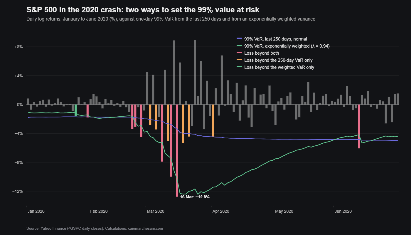
In the 2020 crash it did what it was built for. Over the twenty trading days from 24 February it was broken six times, against eleven for the 250-day version, and by 18 March it stood at 12.4 per cent while the 250-day VaR was still at 4.0 per cent. In the independence test above it scores 8.2 on the S&P 500 against 26.0, and on Bitcoin it passes, at 1.8. Clustering is mostly what it fixes.
It does not fix the frequency. Over the whole period it is broken on 2.1 per cent of days, worse than the historical version. The reason is the other side of reacting quickly: in calm spells it shrinks just as fast, so the first bad day after a quiet month breaks it. On 27 January 2020 it was set at 1.16 per cent and the index fell 1.59 per cent, a day the slower 250-day VaR of 1.71 per cent absorbed. The same thing happened on 5 November 2026: both VaRs were near 1.9 per cent that morning and the index fell 4.45 per cent. The next evening the weighted VaR had jumped to 3.12 per cent, about $30,700 on $1 million, while the 250-day versions barely moved.
Ten days is not ten one-days
Regulatory VaR is quoted over ten trading days, and the usual shortcut is to scale the one-day number by the square root of ten. That is exact only if days are independent and identically distributed, the random-walk assumption I tested in the piece on Brownian motion.
I split the S&P 500 into 903 separate ten-day periods and compared each period’s total return with ten-day VaR set as √10 times the one-day 99 per cent VaR on its first morning. A correct model would be broken in about nine of them. The 250-day normal version was broken in 19, 2.1 per cent of periods. The weighted version was broken in 16, 1.8 per cent. At ten days, as at one, the model is broken about twice as often as it promises. Scaling by √10 assumes that a bad Monday says nothing about Tuesday, and the losses that matter come in runs.
How a regulator would have scored it
The Basel Committee’s 1996 backtesting framework sorts a bank’s 99 per cent VaR model by the number of exceptions in the last 250 days. Up to four is the green zone. Five to nine is yellow, and the bank holds more capital. Ten or more is red, and the model is presumed to be wrong.
The first chart applies that test every day. The normal VaR on the S&P 500 was green on 49 per cent of days, yellow on 31 per cent and red on 20 per cent. It peaked at 26 exceptions in the 250 days to 1 December 2008, ten times the 2.5 expected. Since then it has been red in 2011 to 2012, 2015, 2018 to 2019, 2020 to 2021, 2022 to 2023 and briefly in 2025. A bank running this model on a portfolio that tracked the index would have spent one day in five being told it was broken.
How I use it
As a scale, not as a limit. A one-day 99 per cent VaR is a quick way to say how much a position can move on a bad day in today’s conditions. In the first week of November 2026 it was 2.0 per cent for the S&P 500 on either 250-day method, 3.1 per cent on the weighted one after the fall on 5 November, and between 4.5 per cent and 4.7 per cent for Bitcoin. I look at the 250-day and the weighted figures together. When they diverge, as they did that week, the weighted one is telling me the regime may be changing and the slow one is telling me how much of a change it would take to matter.
What I do not do is treat the 99 per cent number as the worst case. The expected shortfall on 6 November was 2.42 per cent, about $23,900 on $1 million, and the data says even that is the average bad day, not the worst one. I size positions so that a loss of one and a half times the VaR, several days in a row, is survivable, which is the arithmetic behind the piece on how much to risk on a trade. And when exceptions start to arrive in clusters, I read that as the model telling me the regime has changed, not as bad luck.
The S&P 500 had two exceptions in the 250 days to 6 November 2026, comfortably green. It had four at the start of 2020, and between three and five through the first half of 2007. A low count says the last year was calm. It does not say anything about the next one.
Checking it yourself
Every figure above comes from the script below, apart from the 1.15 and 2.338 for a normal distribution, the half-life of the weights, and the dollar amounts, which are arithmetic on its output. It needs pandas, numpy and yfinance, and the two tests are written out by hand.
import numpy as np
import pandas as pd
import yfinance as yf

px = yf.download(["^GSPC", "BTC-USD"], start="1989-12-29", end="2026-11-08",
                 progress=False)["Close"]
WINDOW, Z = 250, {95: 1.645, 99: 2.326}


def backtest(close, level):
    """Yesterday's one-day VaR, two ways, and today's return, all in per cent."""
    r = np.log(close.dropna()).diff().dropna() * 100
    normal = -Z[level] * r.rolling(WINDOW).std().shift(1)
    hist = r.rolling(WINDOW).quantile(1 - level / 100).shift(1)
    keep = normal.notna()
    return r[keep], {"normal": normal[keep], "historical": hist[keep]}


for name, col in (("S&P 500", "^GSPC"), ("Bitcoin", "BTC-USD")):
    for level in (95, 99):
        r, var = backtest(px[col], level)
        if level == 95:
            print(f"{name}: {len(r):,} days from {r.index[0]:%d %b %Y}")
        for method, v in var.items():
            hit = r < v
            worst = (r - v)[hit].idxmin()
            print(f"  {level}% {method:10}: {hit.sum():4} exceptions, {hit.mean():.1%}"
                  f" of days against {100 - level}%; average loss {(r / v)[hit].mean():.2f}"
                  f" x VaR; worst {worst:%d %b %Y}, {r[worst]:.1f}% against {v[worst]:.1f}%")

r, var = backtest(px["^GSPC"], 99)
hit = r < var["normal"]
count = hit.rolling(WINDOW).sum().dropna()
print(f"S&P 500, 99% normal, exceptions in the last {WINDOW} days:",
      f"0 to 4 on {(count <= 4).mean():.0%} of days, 5 to 9 on",
      f"{((count >= 5) & (count <= 9)).mean():.0%}, 10 or more on {(count >= 10).mean():.0%};",
      f"most {count.max():.0f} ({count.idxmax():%d %b %Y})")
days = np.flatnonzero(hit.to_numpy())
print(f"  within five days of the one before: {(np.diff(days) <= 5).mean():.0%}",
      f"of exceptions; {1 - 0.99 ** 5:.0%} if they were independent")
full = hit.loc["1991":"2025"]                    # whole calendar years only
by_year = full.groupby(full.index.year).sum()
print(f"  full years 1991-2025: none in {', '.join(map(str, by_year.index[by_year == 0]))};",
      "most:", ", ".join(f"{y} {n}" for y, n in by_year.nlargest(5).items()))

# Going further: formal tests, a faster model, ten days and expected shortfall
LAMBDA = 0.94                                    # RiskMetrics decay


def returns(close):
    return np.log(close.dropna()).diff().dropna() * 100


def ewma(close, level):
    """One-day VaR from an exponentially weighted variance, started on the first year."""
    r = returns(close)
    s2, out = r.iloc[:WINDOW].var(), []
    for x in r.iloc[WINDOW:]:
        out.append(-Z[level] * np.sqrt(s2))
        s2 = LAMBDA * s2 + (1 - LAMBDA) * x * x
    return r.iloc[WINDOW:], pd.Series(out, index=r.index[WINDOW:])


def kupiec(hit, p):
    """Likelihood ratio for the share of exceptions; above 3.84 rejects at 5%."""
    T, x = len(hit), int(hit.sum())
    q = x / T
    return -2 * ((T - x) * np.log((1 - p) / (1 - q)) + x * np.log(p / q))


def christoffersen(hit):
    """Likelihood ratio for independence, and P(exception | exception yesterday)."""
    h = np.asarray(hit, int)
    a, b = h[:-1], h[1:]
    n = {(i, j): int(((a == i) & (b == j)).sum()) for i in (0, 1) for j in (0, 1)}
    p01 = n[0, 1] / (n[0, 0] + n[0, 1])
    p11 = n[1, 1] / (n[1, 0] + n[1, 1])
    p = (n[0, 1] + n[1, 1]) / len(a)
    ll = lambda k, pr: k * np.log(pr) if k else 0.0
    lr = -2 * (ll(n[0, 0] + n[1, 0], 1 - p) + ll(n[0, 1] + n[1, 1], p)
               - ll(n[0, 0], 1 - p01) - ll(n[0, 1], p01)
               - ll(n[1, 0], 1 - p11) - ll(n[1, 1], p11))
    return lr, p11


print("99% one-day VaR    share   Kupiec  Christoffersen  P(again next day)  loss/VaR")
for name, col in (("S&P 500", "^GSPC"), ("Bitcoin", "BTC-USD")):
    r, var = backtest(px[col], 99)
    var["EWMA"] = ewma(px[col], 99)[1]
    for method, v in var.items():
        hit = r < v
        lr_ind, again = christoffersen(hit)
        print(f"{name:8} {method:10} {hit.mean():5.1%}  {kupiec(hit, 0.01):7.1f}"
              f"  {lr_ind:14.1f}  {again:17.0%}  {(r / v)[hit].mean():8.2f}")

r, var = backtest(px["^GSPC"], 99)
e = ewma(px["^GSPC"], 99)[1]
crash = slice("2020-02-24", "2020-03-20")
print(f"S&P 500, 24 Feb to 20 Mar 2020: normal {(r < var['normal'])[crash].sum()},"
      f" EWMA {(r < e)[crash].sum()} exceptions in {len(r[crash])} days;"
      f" VaR on 21 Feb {var['normal']['2020-02-21']:.2f} and {e['2020-02-21']:.2f},"
      f" on 18 Mar {var['normal']['2020-03-18']:.2f} and {e['2020-03-18']:.2f}")

ten = r.groupby(np.arange(len(r)) // 10)
blocks = pd.DataFrame({"loss": ten.sum(), "start": ten.apply(lambda s: s.index[0])})
blocks = blocks[ten.size() == 10]
for method, v in (("normal", var["normal"]), ("EWMA", e)):
    hit = blocks.loss.to_numpy() < np.sqrt(10) * v[blocks.start].to_numpy()
    print(f"Ten-day 99% VaR by the square root of 10, {method}: {hit.sum()} of {len(hit)}"
          f" ten-day periods, {hit.mean():.1%}")

r = returns(px["^GSPC"])
q975 = r.rolling(WINDOW).quantile(0.025).shift(1)
es = r.rolling(WINDOW).apply(lambda w: np.sort(w)[:6].mean(), raw=True).shift(1)
ok = q975.notna()
r, q975, es = r[ok], q975[ok], es[ok]
hit = r < q975
print(f"97.5% historical VaR: {hit.mean():.1%} of days; average loss on those days {r[hit].mean():.2f}%"
      f" against a forecast expected shortfall of {es[hit].mean():.2f}%")
print(f"6 Nov 2026: one-day 99% VaR normal {var['normal'].iloc[-1]:.2f}%, historical"
      f" {var['historical'].iloc[-1]:.2f}%, EWMA {e.iloc[-1]:.2f}%; 97.5% expected shortfall"
      f" {r.iloc[-WINDOW:].sort_values().iloc[:6].mean():.2f}%")
Run in November 2026 it prints:
S&P 500: 9,031 days from 27 Dec 1990
  95% normal    :  469 exceptions, 5.2% of days against 5%; average loss 1.54 x VaR; worst 16 Mar 2020, -12.8% against -2.4%
  95% historical:  480 exceptions, 5.3% of days against 5%; average loss 1.57 x VaR; worst 16 Mar 2020, -12.8% against -1.9%
  99% normal    :  208 exceptions, 2.3% of days against 1%; average loss 1.42 x VaR; worst 16 Mar 2020, -12.8% against -3.4%
  99% historical:  145 exceptions, 1.6% of days against 1%; average loss 1.38 x VaR; worst 16 Mar 2020, -12.8% against -4.8%
Bitcoin: 4,184 days from 26 May 2015
  95% normal    :  181 exceptions, 4.3% of days against 5%; average loss 1.58 x VaR; worst 12 Mar 2020, -46.5% against -5.3%
  95% historical:  220 exceptions, 5.3% of days against 5%; average loss 1.68 x VaR; worst 12 Mar 2020, -46.5% against -4.8%
  99% normal    :   82 exceptions, 2.0% of days against 1%; average loss 1.47 x VaR; worst 12 Mar 2020, -46.5% against -7.5%
  99% historical:   56 exceptions, 1.3% of days against 1%; average loss 1.40 x VaR; worst 12 Mar 2020, -46.5% against -10.0%
S&P 500, 99% normal, exceptions in the last 250 days: 0 to 4 on 49% of days, 5 to 9 on 31%, 10 or more on 20%; most 26 (01 Dec 2008)
  within five days of the one before: 35% of exceptions; 5% if they were independent
  full years 1991-2025: none in 2003, 2004, 2009, 2023; most: 2008 25, 2007 15, 2018 15, 2022 15, 2020 14
99% one-day VaR    share   Kupiec  Christoffersen  P(again next day)  loss/VaR
S&P 500  normal      2.3%    113.2            26.0                 9%      1.42
S&P 500  historical  1.6%     28.3            21.4                 8%      1.38
S&P 500  EWMA        2.1%     90.5             8.2                 6%      1.38
Bitcoin  normal      2.0%     30.4             7.5                 7%      1.47
Bitcoin  historical  1.3%      4.4             4.0                 5%      1.40
Bitcoin  EWMA        2.2%     42.1             1.8                 4%      1.54
S&P 500, 24 Feb to 20 Mar 2020: normal 11, EWMA 6 exceptions in 20 days; VaR on 21 Feb -1.74 and -1.56, on 18 Mar -3.97 and -12.40
Ten-day 99% VaR by the square root of 10, normal: 19 of 903 ten-day periods, 2.1%
Ten-day 99% VaR by the square root of 10, EWMA: 16 of 903 ten-day periods, 1.8%
97.5% historical VaR: 3.2% of days; average loss on those days -2.82% against a forecast expected shortfall of -2.78%
6 Nov 2026: one-day 99% VaR normal -1.99%, historical -1.96%, EWMA -3.12%; 97.5% expected shortfall -2.42%