
Shell and BP are the textbook pair in London. Two integrated oil majors in the FTSE 100, selling much the same products into the same markets and moved by the same oil price. If any two shares ought to move together, these two should, and day to day they do: over the sixteen years to October 2026 their daily returns had a correlation of 0.81.
Over the same sixteen years, with dividends reinvested, Shell returned 111 per cent and BP returned 3 per cent.
Both numbers are true, and the distance between them is what pairs trading is about. In my piece on relative value against directional trading I used Brent and WTI crude to show what a spread trade looks like. This is the same idea applied to two shares, worked through on real prices: the test that tells you whether a pair can be traded at all, a rule that only uses what was known at the time, and the costs that decide whether any of it pays.
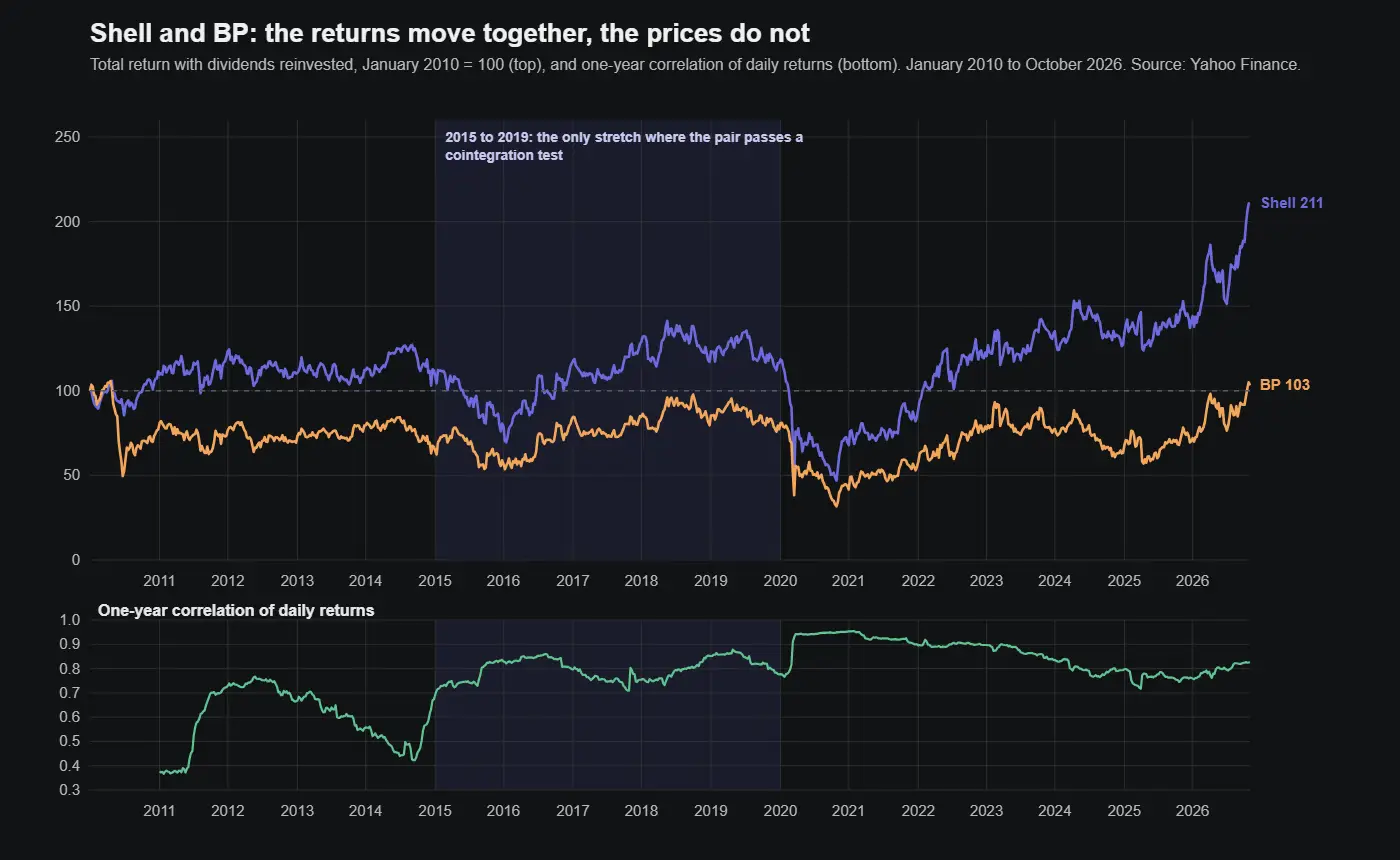
Correlation is about returns, cointegration is about prices
Correlation measures whether two shares move in the same direction on the same day. It says nothing about whether their prices stay together. Two shares can rise and fall together on most days and still drift apart for good, if one of them grows a little faster on average, or falls a little further each time the sector has a bad week. Over sixteen years a small difference in drift becomes the difference between 111 per cent and 3 per cent.
A pairs trade is a bet on prices. You buy the share that looks cheap against the other and sell the one that looks expensive, and you make money only if the gap closes. What you need is a combination of the two prices, Shell minus some multiple of BP, that keeps coming back to an average. The statistical name for that is cointegration, and the property that matters is that the gap is pulled back towards its average rather than wandering off.
The standard check is the two-step test of Engle and Granger. Regress the log price of one share on the log price of the other, take what is left over (the residual, which is the spread you would trade), and test whether that residual reverts with an augmented Dickey-Fuller test. The test gives a statistic: the more negative it is, the stronger the evidence. For a pair of prices the 5 per cent threshold is about −3.34 and the 1 per cent threshold about −3.90. The same regression gives the hedge ratio, how much BP to hold against each pound of Shell, and the speed of reversion can be turned into a half-life, the number of trading days it takes for a gap to close by half.
What the test says about Shell and BP
| Period | Hedge ratio | Correlation of daily returns | Test statistic | Half-life, trading days |
|---|---|---|---|---|
| 2010 to 2014 | 0.10 | 0.56 | −2.83 | 61 |
| 2015 to 2019 | 0.99 | 0.81 | −4.53 | 25 |
| 2020 to 2021 | 0.92 | 0.94 | −1.47 | 77 |
| 2022 to October 2026 | 0.73 | 0.83 | −1.40 | 223 |
| Whole period | 0.94 | 0.81 | −2.92 | 204 |
Only one period passes, and it passes comfortably. From 2015 to 2019 the hedge ratio was close to one, the test statistic was well beyond the 1 per cent threshold and a gap between the two halved in about 25 trading days, five weeks. That is the pair the textbooks describe.
The other periods each fail for a different reason. In 2010 to 2014 the regression finds almost no link between the two price levels, a hedge ratio of 0.10. On 20 April 2010 the Deepwater Horizon rig exploded in the Gulf of Mexico, and by 29 June BP’s shares had fallen 54 per cent, from 655p to 303p. The correlation of daily returns that year was 0.38. A company-specific disaster is exactly the event a pairs trade has no defence against, because only one side of the pair suffers it.
2020 and 2021 are the interesting case. The correlation of daily returns was the highest of any period, 0.94, because both shares fell together in the crash of March 2020 and recovered together. And yet the test fails. Both companies cut their dividends that year, but not by the same amount or at the same time: Shell’s quarterly payment fell from 36.4p a share in February to 12.7p in May, while BP kept its payment in May and halved it, from 8.3p to 4.0p, in August. When two companies choose different dividend policies, the relationship between their share prices moves, however closely they trade from one day to the next.
Since 2022 the two have simply gone their own ways. Shell’s total return index has more than doubled from where it stood at the start of 2022, BP’s has risen by about three-quarters, and a half-life of 223 trading days means there was no reversion anyone could have traded.
One caution about the table. Each row uses that period’s own data to set the hedge ratio, which flatters the result. A trader at the start of 2015 could not have known that the next five years would be the good ones.
A rule that only uses what was known at the time
To see what the pair would actually have paid, I ran a rule that never looks ahead. Each day it regresses the last 252 trading days of Shell’s log price on BP’s and measures how far today’s prices sit from that line, in standard deviations of the past year’s residuals. When the gap is more than two standard deviations, it sells the expensive side and buys the cheap one in the proportion the regression gives. It closes the trade when the gap is back on the line, when it has moved another two standard deviations against (a stop at four), or after 60 trading days. Returns are measured on the total money committed to both sides, with 0.25 per cent taken off each round trip as a placeholder for commission, the bid-offer spread and the cost of borrowing the share that is sold short.
| Trades opened in | Trades | Made money | Average per trade | Total |
|---|---|---|---|---|
| 2010 to 2014 | 11 | 64% | 0.43% | 4.7% |
| 2015 to 2019 | 14 | 64% | 0.77% | 10.8% |
| 2020 to 2021 | 8 | 25% | −0.83% | −6.6% |
| 2022 to October 2026 | 16 | 50% | −0.04% | −0.6% |
| All | 49 | 53% | 0.17% | 8.3% |
Forty-nine trades in sixteen years, about three a year, held for a median of 39 trading days. Only 15 of them closed because the gap came back to the line. Sixteen hit the stop and 18 ran out of time, which is what a weak or absent relationship looks like from the inside: you wait, and the spread neither comes back nor goes far enough to stop you out. Before costs the average trade made 0.42 per cent. After them it made 0.17 per cent, and the total over sixteen years was about 8 per cent on the money committed, before paying for the money itself.
The rule made its money where the test said it would, in 2015 to 2019. It did not know that in advance. It happened to be trading during the years when the relationship held, and it gave most of the gains back in the two years when it did not.
All of this is before tax. Buying UK shares electronically costs 0.5 per cent in Stamp Duty Reserve Tax. A pairs trade buys shares when it opens the long side and again when it buys back the short side, so the tax alone comes to at least 0.25 per cent of the whole position per round trip, which on these numbers would take the entire edge. It is one reason pair traders in London usually hold their positions through derivatives rather than the shares themselves.
What the example teaches
Test for cointegration, and test it on rolling windows rather than once over the whole history. A pair’s relationship has regimes, and a test run over sixteen years averages a good period with three bad ones and tells you about none of them.
Know why the pair should come back together, because the statistics only find out after the fact. Two companies with similar assets, similar strategies and similar payouts should stay together. When one of those stops being true, as with the dividend decisions of 2020, the price relationship changes first and the test catches up a year or two later.
Look at the half-life before the entry signal. It tells you how long you will wait for a trade to work, and if it is longer than your patience, your stop or your financing, the pair is not a trade however attractive the gap looks.
And expect costs to be a large share of the edge in any single pair. That is why desks that do this professionally run dozens of pairs at once and do the trading through instruments that avoid the tax, and why a single textbook pair, traded through the shares, is better used for learning than for income.
Checking it yourself
The whole analysis runs in Python with numpy and the yfinance library. The first part prints the test for each period; the second runs the trading rule.
import numpy as np
import yfinance as yf

px = yf.download(["SHEL.L", "BP.L"], start="2010-01-01", end="2026-10-31", auto_adjust=True)["Close"].dropna()
s, b = np.log(px["SHEL.L"].to_numpy()), np.log(px["BP.L"].to_numpy())
dates = px.index


def eg_test(s, b):
    """Engle-Granger: hedge ratio, ADF t-statistic on the residual, half-life in days."""
    beta, alpha = np.polyfit(b, s, 1)
    e = s - alpha - beta * b
    de = np.diff(e)
    y = de[1:]
    X = np.column_stack([np.ones(len(y)), e[1:-1], de[:-1]])
    coef, *_ = np.linalg.lstsq(X, y, rcond=None)
    resid = y - X @ coef
    s2 = resid @ resid / (len(y) - 3)
    t = coef[1] / np.sqrt(s2 * np.linalg.inv(X.T @ X)[1, 1])
    return beta, t, -np.log(2) / np.log(1 + coef[1])


for lo, hi in [("2010", "2014"), ("2015", "2019"), ("2020", "2021"), ("2022", "2026"), ("2010", "2026")]:
    m = (dates >= f"{lo}-01-01") & (dates <= f"{hi}-12-31")
    beta, t, half_life = eg_test(s[m], b[m])
    print(f"{lo}-{hi}: hedge ratio {beta:.2f}, test statistic {t:.2f}, half-life {half_life:.0f} days")


def pair_rule(s, b, window=252, entry=2.0, stop=4.0, max_days=60, cost=0.0025):
    """Trade the residual of a rolling regression, using only past data."""
    trades, pos = [], 0
    for t in range(window, len(s)):
        if pos:
            pnl += pos * ((s[t] - s[t - 1]) - beta * (b[t] - b[t - 1]))
        bt, at = np.polyfit(b[t - window:t], s[t - window:t], 1)
        sd_t = np.std(s[t - window:t] - at - bt * b[t - window:t], ddof=1)
        if not pos:
            z = (s[t] - at - bt * b[t]) / sd_t
            if abs(z) > entry and bt > 0:
                pos, start, beta, alpha, sd, pnl = -np.sign(z), t, bt, at, sd_t, 0.0
        else:
            z = (s[t] - alpha - beta * b[t]) / sd
            if pos * z >= 0 or pos * z <= -stop or t - start >= max_days:
                trades.append(pnl / (1 + beta) - cost)
                pos = 0
    return np.array(trades)


trades = pair_rule(s, b)
print(f"{len(trades)} trades, {(trades > 0).mean():.0%} winners, "
      f"average {trades.mean():.2%}, total {trades.sum():.1%}")
Yahoo’s adjusted prices include dividends and are revised from time to time, so expect small differences from the figures above. The rule takes a few minutes to run, because it fits a new regression every day.