
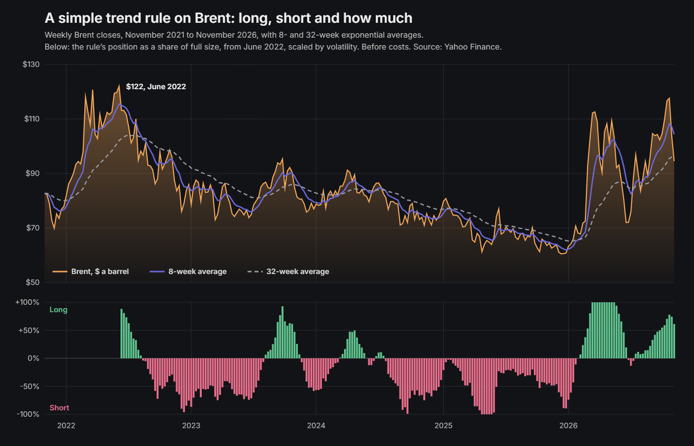
In June 2022 Brent crude closed at $122 a barrel, its highest weekly close in the last five years. A simple trend rule of the kind I describe below was close to its largest long position. By the middle of August, with Brent at $96.70, the same rule had turned short. Nobody decided either of those things. That is the idea behind a systematic macro fund, and it is also where most explanations of one stop.
This is the longer version: what such a fund actually does each week, in the order it does it, with the arithmetic. The fund I founded in London was a quantitative macro fund with a bias towards energy, trading futures and options alongside currencies and equity indices. What follows is the general shape of the business, not a description of that fund’s models.
What “systematic” and “macro” each mean
Macro describes what is traded: the large, liquid markets that move with growth, inflation, interest rates and supply. Government bond and interest rate futures, currencies, equity index futures and commodities. Not individual companies.
Systematic describes how the decisions are made. The views are written down as rules, in code, and tested on history before any money depends on them. A person decides the rules. The rules decide the trades. A discretionary macro manager reads the same central bank statement and decides what to do about it; a systematic one decided months earlier what any statement of that kind would be allowed to change.
The practical difference is that every decision a systematic fund makes can be replayed. If a position lost money, you can see exactly which input caused it, and whether the rule did what it was built to do. That is uncomfortable, and it is the point.
Four jobs, in order
Every week, or every day, or every few minutes depending on the fund, the same four things happen:
- Turn prices and data into a forecast for each market.
- Turn each forecast into a position size.
- Check that the positions together carry the risk the fund intends, and no more.
- Trade, without giving the edge away in costs.
People outside the industry assume the first job is the clever part. Most of the work, and most of the failures, are in the other three.
Job one: a forecast you can compare across markets
Forecasts come from a small number of families. Trend: prices that have been rising tend to keep rising for a while. Carry: what you earn or pay just for holding a position, such as the roll on a futures curve or the interest rate gap between two currencies. Value or mean reversion: prices that have moved too far from some anchor tend to come back. And fundamentals: a model of supply and demand. In energy that last one is where a specialist earns their place, because a refinery model that tells you whether a price is supported by margins (I explained the main one in the piece on the crack spread) fails at different times from a moving average.
Take the simplest trend rule there is. Compare a fast exponential average of the price with a slow one. Here the fast one covers about 8 weeks and the slow one about 32. When the fast average is above the slow one, the trend is up.
The gap between the two is in dollars, and a dollar gap means different things in a calm market and a wild one. So the gap is divided by the size of a normal weekly move. That turns it into a number you can compare between Brent, the euro and the S&P 500.
In the first week of November 2026 Brent was $94.50. The 8-week average was $104.30 and the 32-week average $95.90, a gap of $8.40. Over the previous 26 weeks Brent’s volatility was 52.5% a year, which makes a normal weekly move about $6.88 (94.50 × 0.525 ÷ √52). The forecast is 8.40 ÷ 6.88 ≈ 1.2.
Notice that the price has already fallen below the slow average, and the rule is still long. That lag is not a fault. It is the price of not reacting to every move, and you cannot have a trend rule without it.
Carry works the same way, with different inputs. Suppose the front Brent contract is $94.50 and the contract three months later is $92.00. A long position that keeps rolling forward picks up about $2.50 a quarter if nothing else changes: 2.50 ÷ 94.50 × 4 ≈ 10.6% a year. Divide that by volatility and it becomes another forecast on the same scale as the trend one, and the two can be added.
Job two: size by risk, not by conviction
A forecast says which way. It does not say how much. The size comes from the risk budget.
Say the fund has $100 million and wants its returns to move by about 10% a year, no more. Spread across 25 markets that behave roughly independently, each market gets about 2% of that (10% ÷ √25), or $2 million a year of risk.
One Brent futures contract is 1,000 barrels: at $94.50, that is $94,500 of oil. At 52.5% volatility, one contract carries about $49,600 a year of risk (94,500 × 0.525). A full position is therefore about 40 contracts ($2,000,000 ÷ 49,600).
The forecast then scales that full position. Here the rule is to halve the forecast and cap the result at one full position either way. A forecast of 1.2 gives 0.61 of full size: about 25 contracts long.
The important consequence is what happens when volatility changes. In August 2024 Brent’s volatility was 20.7%. At today’s price, a full position at that volatility would be about 100 contracts. In August 2026 it reached 67.5%, and a full position would be about 31. The fund holds three times as many barrels in a calm market as in a wild one, for the same risk. Measuring volatility properly is therefore not an academic exercise; the average true range is one way to do it, the standard deviation of returns used here is another.
Job three: the book is not the sum of the trades
The 2% per market assumed the markets were independent. They are not. Brent, WTI, gasoil, gasoline and heating oil move together, so five long oil positions are closer to one large bet than to five small ones.
The arithmetic is short. Two positions with 2% of risk each and a correlation of 0.9 carry about 3.9% together (2% × √(1 + 1 + 2 × 0.9)). If they were independent, it would be about 2.8%. The fund calculates the risk of the whole book from the correlations between every pair of markets, and scales everything down if the total is above target.
The hard part is that correlations are not constant. They tend to rise exactly when markets fall, which is when diversification is needed most. I wrote about how unstable the number is in the piece on correlation. A fund that measures correlation over calm months and trusts it in a crisis is carrying more risk than its own report says.
Job four: trading without paying the edge away
Futures expire, so every position has to be rolled into the next contract on a schedule, usually some days before the expiry when most of the market is rolling too. Every trade costs half the bid-offer spread, a commission, and in larger sizes some market impact. A rule that changes its mind every week pays those costs fifty times a year; a slower one pays them a few times.
The common fix is a buffer. The fund only trades when the target position is far enough from the current one to be worth it, say more than 10% of full size. If the target is 25 contracts and the fund holds 23, the difference is 2 contracts, 5% of a 40-contract full position, and nothing happens. Most of the small weekly changes in a forecast never become trades. Execution then concentrates on the most liquid hours, when the spread is tightest.
What the example does when you run it
The chart above is that rule on five years of weekly Brent prices. It needs about 32 weeks of history before it can start, so it begins trading in June 2022. From then to early November 2026 it was long for 77 weeks and short for 154, and changed direction 10 times. Before costs, it lost about 5.4% a year, with returns moving by about 6.8% a year.
The reason is in the chart. From early 2023 to the end of 2025 Brent traded between about $60 and $95, with no trend long enough to pay for the lag. The rule bought rallies after they had started and sold falls after they had started, and each time the market turned back. Even 2026 did not rescue it. The rule caught most of the jump from $72 to $112 in March, and gave all of it back by the end of June as the price fell to $72 again.
It is not a bad choice of settings. A faster version, 4 and 16 weeks, lost about 3.5% a year and changed direction 22 times. A slower one, 16 and 64 weeks, lost about 6.2% a year. Simply holding Brent, sized the same way by volatility, made roughly nothing over the same period.
That is not an argument against trend following. It is the reason nobody runs it on one market. The long evidence for trend comes from many markets at once: Hurst, Ooi and Pedersen at AQR simulated a trend strategy across a broad set of markets back to 1880 and found it consistently profitable over more than a century. Any one market can go years without a usable trend. Twenty-five uncorrelated ones rarely all do, and the losses in the quiet markets are paid for by the few that move.
What a systematic fund cannot do
It cannot read the news. When a war starts or an OPEC meeting goes badly, the rules know about it only when the price moves, and by then the first part of the move has happened.
It cannot tell that the world has changed until enough data says so. A rule tested on twenty years of one kind of market will keep behaving as though that market still exists.
And it is easy to fool yourself in testing. With enough parameters you can fit any history perfectly and learn nothing. The defences are dull: few parameters, results that hold for neighbouring settings (as the three versions above do, in the wrong direction), and a stretch of data the model never saw while it was being built. If a strategy only works at exactly 8 and 32 weeks, it does not work.
The useful way to think about it is that a systematic fund is a set of decisions made calmly in advance, about situations that will not be calm. The quality of the fund is the quality of those decisions, and the honesty with which they are tested. I compared the two broad styles of trading, betting on direction and betting on the gap between two prices, in the piece on relative value and directional trading; a systematic macro fund usually does some of both.
Running it yourself
The weekly futures prices are free. In Python, with the yfinance library, the whole rule is a few lines:
import numpy as np
import yfinance as yf

px = yf.download("BZ=F", start="2021-11-01", interval="1wk")["Close"].squeeze()
fast = px.ewm(span=8).mean()
slow = px.ewm(span=32).mean()
vol = np.log(px).diff().rolling(26).std() * np.sqrt(52)

forecast = (fast - slow) / (px * vol / np.sqrt(52))
position = (forecast / 2).clip(-1, 1)          # share of a full position
weekly = position.shift(1) * 0.10 / vol.shift(1) * np.log(px).diff()

print(weekly.mean() * 52, weekly.std() * np.sqrt(52))
The last line prints the annual return and annual volatility of the rule before costs. Change the spans, add a second market, and you will see quickly why the work is in jobs two to four. Front-month futures roll from one contract to the next, which puts small jumps into a continuous price series, so treat any single week with some caution.